Table of Contents
- 1 Problem Statement
- 2 Analysis Approach & Conclusions
- 3 Importing data
- 4 Data Quality Checks
- 5 Exploratory Data Analysis
- 5.1 Univariate Analysis / Outlier Treatment
- 5.2 Bivariate Analysis
- 5.2.1 Pairplot
- 5.2.2 Child Mortality vs Life Expectancy
- 5.2.3 Child Mortality vs Total Fertility
- 5.2.4 GDP per capita vs Health Spending
- 5.2.5 Imports vs GDP per capita
- 5.2.6 Exports vs GDP per capita
- 5.2.7 GDP per capita vs Trade Deficit
- 5.2.8 Net Income per person vs Inflation
- 5.2.9 GDP per capita vs Inflation
- 5.3 Correlation Analysis
- 6 Hopkin's Statistic
- 7 Standardizing Values
- 8 K-Means Clustering
- 9 Hierarchical Clustering
- 10 Mixed K-Means Clustering
- 11 Cluster Profiling
- 12 Conclusion
HELP - Countries to Aid
Jayanth Boddu
Clustering
Problem Statement
An NGO wants to use their funding strategically so that they could aid five countries in dire need of help. The analyst’s objective is to use clustering algorithms to group countries based on socio-economic and health factors to judge the overall development of countries. Further,the final deliverable is - suggesting 5 countries that need the aid the most.
Analysis Approach & Conclusions
- The objective of the analysis is to recommend 05 countries in dire need of aid of help.
- The achieve this, the following features of 167 countries have been analyzed.
- GDP per capita
- Child mortality per 1000 live births
- Net Income per person
- Fertility rates at the current previaling age/fertility rate
- Inflation index
- Life Expectancy
- Imports per capita
- Exports per capita
- Total Health Spending per capita
- The above features are further grouped into health, economic and policy indicators
- Health Indicators
- Child mortality per 1000 births
- Fertility rates at the current previaling age/fertility index
- Life Expectancy
- Economic Indicators
- Net Income per person
- Imports per capita
- Exports per capita
- Inflation Index
- Policy Indicators
- Total Health Spending per capita
- Health Indicators
- From the above, countries deduced to be in dire need of aid are countries with bad economic indicators and bad health indicators having low health spending
- Further on the feature level, the following are general indicators of need of aid.
| Feature | High / Low |
| Child Mortality | High |
| Life Expectancy | Low |
| Fertility | High |
| Health Spending | Low |
| GDP per capita | Low |
| Inflation Index | High |
| Income per Person | Low |
| Imports | High |
| Exports | Low |
Data has been check for quality.No Data Quality Issues have been found - No missing values, No duplicates , No incorrect data types
A new feature ‘Trade Deficit’ has been derived.
- Trade Deficit = Imports - Exports
- Trade Deficit or Trade balance is a good indicator of economic health of countries with low GDP per capita
- Lower or negative is better than higher and positive.
Univariate analysis revealed the following information
| Feature | Highest | Lowest |
| Child Mortality | Haiti,Sierra Leone | Iceland |
| Life Expectancy | Japan , Singapore | Haiti, Lesotho |
| Total fertility | Chad, Niger | Singapore, South Korea |
| Health Spending | Switzerland, US | Madagascar, Eritrea |
| GDP per capita | Luxemborg , Norway | Burundi , Liberia |
| Inflation Index | Nigeria, Venezuela | Seycelles, Ireland |
| Net Income per person | Qatar, Luxemborg | Liberia, Congo Dem. Rep. |
| Imports per capita | Luxemborg, Singapore | Myanmar, Burundi |
| Exports per capita | Luxemborg, Singapore | Myanmar, Burundi |
| Trade Deficit per capita | Bahamas, Greece | Luxemborg, Qatar |
- Since there’s less data per cluster, soft range of 1st percentile - 99th perentile has been used to classify and cap outliers. Only those outliers which do not skew the areas of interest have been capped.
- Outlier Treatment Summary
| Feature | Upper Outliers | Lower Outliers |
| Child Mortality | Not Changed | Capped |
| Life Expectancy | Capped | Not Changed |
| Fertility | Not Changed | Capped |
| Health Spending | Capped | Not Capped |
| GDP per capita | Capped | Not Changed |
| Inflation Index | Not Changed | Capped |
| Income per Person | Capped | Not Changed |
| Imports | Capped | Not Changed |
| Exports | Capped | Not Changed |
- Bivariate Analysis revealed the following insights
- There is a negative relationship between Child Mortality and Life expectancy. As child mortality increases, Life Expectancy decreases. Haiti and Sierra Leone have the highest child mortality and lowest life expectancy.
- There is positive relationship between child mortality and total fertility. Ex : Chad and Mali
- Health Spending has a positive relationship with GDP per capita , but the situation is dire in case of low GDP countries like Eritrea & Madagascar.
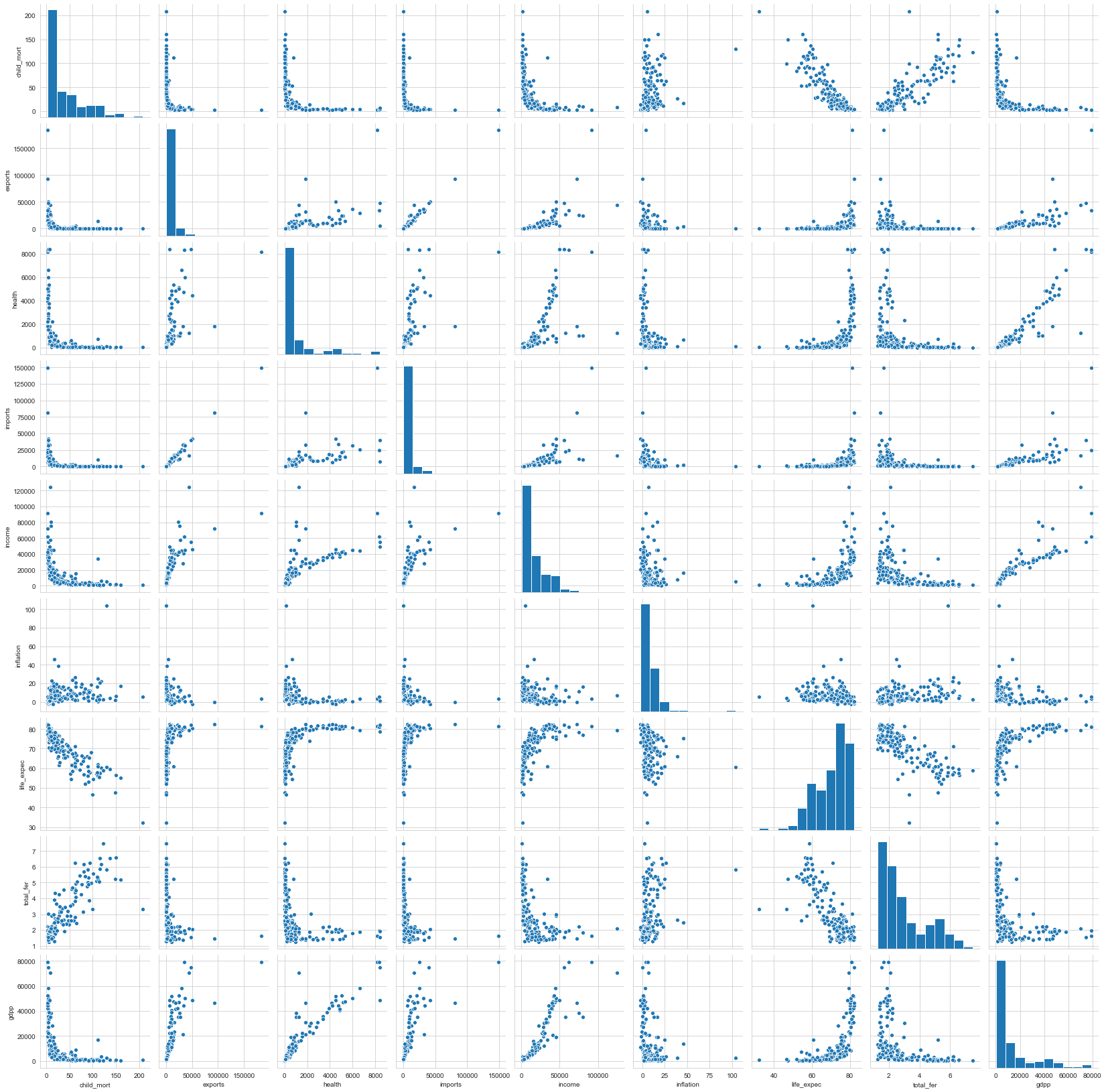
- There’s very high correlation between child mortality and life expectancy , child mortality and total fertility.
Columns : ‘child_mort’, ‘exports’, ‘health’, ‘imports’, ‘income’,‘inflation’, ‘life_expec’, ‘total_fer’, ‘gdpp’,‘trade_deficit’ were used for clustering.
Hopkin’s Statistic was calculated which showed a very high mean clustering tendency of 96% with a standard deviation of 4%
The dataset was standardized with mean = 0 , standard deviation = 1 before clustering.
Optimum no of clusters for k-means was found to be 4 , both from Elbow curve and Silhoeutte Analysis curve.
Clustering with k-means was performed (Cluster centers initialized with k-means++)
Hierarchical Clustering with Single, Complete and Average linkages and Euclidean , correlation based distances were explored.
Mixed Clustering - K-Means clustering initialised with centroids of Hierarchical clusters , 6 no of clusters - was carried out.
Finally, Hierarchical Clustering with Complete linkage and correlation based distance measure was chosen to arrive at the results. Choice was made based on interpretability of results.
Characteristics of Clusters obtained :
| Cluster | GDP | Income | Child Mortality |
| 0 | Very low | Very Low | Very High |
| 1 | low | low | low |
| 2 | Moderate | Moderate | Moderate |
| 3 | High | High | Low |
| 4 | Very High | Very High | Low |
| 5 | Very Low | Very Low | Low |
- From the characteristics , we see that the Cluster 0 is our area of interest.
- According to the UN goals of 2030, the top priority is health and then poverty.
- Hence countries in cluster 0 were ranked based on Child Mortality followed by income and GDP per capita.
- By that criteria, the following are the five countries HELP should consider extending their aid.
- Haiti
- Sierra Leone
- Chad
- Central African Republic
- Mali
1import numpy as np2import pandas as pd3import matplotlib.pyplot as plt45import seaborn as sns6sns.set_style('whitegrid')78from sklearn.cluster import KMeans9from scipy.cluster.hierarchy import linkage10from scipy.cluster.hierarchy import dendrogram11from scipy.cluster.hierarchy import cut_tree1213import warnings14warnings.filterwarnings('ignore')1516!pip install tabulate17!jt -f roboto -fs 12 -cellw 100%1819from tabulate import tabulate2021from bokeh.models import ColumnDataSource, HoverTool22from bokeh.plotting import figure,show,output_notebook,reset_output23from bokeh.transform import factor_cmap24from bokeh.layouts import row25output_notebook()
1Requirement already satisfied: tabulate in /Users/jayanth/opt/anaconda3/lib/python3.7/site-packages (0.8.7)
1# to table print a dataframe2def tab(ser) :3 print(tabulate(pd.DataFrame(ser), headers='keys', tablefmt='psql'))
Importing data
1countries = pd.read_csv('./Country-data.csv')2tab(countries.head())
1+----+---------------------+--------------+-----------+----------+-----------+----------+-------------+--------------+-------------+--------+2| | country | child_mort | exports | health | imports | income | inflation | life_expec | total_fer | gdpp |3|----+---------------------+--------------+-----------+----------+-----------+----------+-------------+--------------+-------------+--------|4| 0 | Afghanistan | 90.2 | 10 | 7.58 | 44.9 | 1610 | 9.44 | 56.2 | 5.82 | 553 |5| 1 | Albania | 16.6 | 28 | 6.55 | 48.6 | 9930 | 4.49 | 76.3 | 1.65 | 4090 |6| 2 | Algeria | 27.3 | 38.4 | 4.17 | 31.4 | 12900 | 16.1 | 76.5 | 2.89 | 4460 |7| 3 | Angola | 119 | 62.3 | 2.85 | 42.9 | 5900 | 22.4 | 60.1 | 6.16 | 3530 |8| 4 | Antigua and Barbuda | 10.3 | 45.5 | 6.03 | 58.9 | 19100 | 1.44 | 76.8 | 2.13 | 12200 |9+----+---------------------+--------------+-----------+----------+-----------+----------+-------------+--------------+-------------+--------+
- The dataset contains
exports,imports,healthas a proportion of GDP per capita - Let’s convert them to actual values
1# conversion to actual values2countries['exports'] = 0.01 * countries['exports'] * countries['gdpp']3countries['imports'] = 0.01 * countries['imports'] * countries['gdpp']4countries['health'] = 0.01 * countries['health'] * countries['gdpp']
Data Quality Checks
1tab(countries.info())
1<class 'pandas.core.frame.DataFrame'>2RangeIndex: 167 entries, 0 to 1663Data columns (total 10 columns):4 # Column Non-Null Count Dtype5--- ------ -------------- -----6 0 country 167 non-null object7 1 child_mort 167 non-null float648 2 exports 167 non-null float649 3 health 167 non-null float6410 4 imports 167 non-null float6411 5 income 167 non-null int6412 6 inflation 167 non-null float6413 7 life_expec 167 non-null float6414 8 total_fer 167 non-null float6415 9 gdpp 167 non-null int6416dtypes: float64(7), int64(2), object(1)17memory usage: 13.2+ KB
- 167 countries
- No apparent missing values
- No incorrect data types
1# taking a closer look to see if any country is duplicated2countries[countries.duplicated(subset=['country'])].index.values
1array([], dtype=int64)
- No duplicate countries
1# exports, health, imports are a percentage of GDPP . Checking if there are any anomalies2condition1 = countries['health'] < countries['gdpp']3condition2 = countries['imports'] < countries['gdpp']4condition3 = countries['exports'] < countries['gdpp']56# countries which don't satisfy the above conditions7index = countries[~(condition1 & condition2 & condition3)].index.values8countries.loc[index]
| country | child_mort | exports | health | imports | income | inflation | life_expec | total_fer | gdpp | |
| 73 | Ireland | 4.2 | 50161.00 | 4475.53 | 42125.5 | 45700 | -3.220 | 80.4 | 2.05 | 48700 |
| 87 | Lesotho | 99.7 | 460.98 | 129.87 | 1181.7 | 2380 | 4.150 | 46.5 | 3.30 | 1170 |
| 91 | Luxembourg | 2.8 | 183750.00 | 8158.50 | 149100.0 | 91700 | 3.620 | 81.3 | 1.63 | 105000 |
| 98 | Malta | 6.8 | 32283.00 | 1825.15 | 32494.0 | 28300 | 3.830 | 80.3 | 1.36 | 21100 |
| 131 | Seychelles | 14.4 | 10130.40 | 367.20 | 11664.0 | 20400 | -4.210 | 73.4 | 2.17 | 10800 |
| 133 | Singapore | 2.8 | 93200.00 | 1845.36 | 81084.0 | 72100 | -0.046 | 82.7 | 1.15 | 46600 |
- Some countries have greater imports than GDP per capita
1# child mortality rate is calculated for 1000 live births. Let's check if its above 10002countries[countries['child_mort'] > 1000].index.values
1array([], dtype=int64)
- Sanity checks completed.
- No Data Quality issues found.
Exploratory Data Analysis
1# summary statistics2tab(countries.describe())
1+-------+--------------+--------------+-----------+---------------+----------+-------------+--------------+-------------+----------+2| | child_mort | exports | health | imports | income | inflation | life_expec | total_fer | gdpp |3|-------+--------------+--------------+-----------+---------------+----------+-------------+--------------+-------------+----------|4| count | 167 | 167 | 167 | 167 | 167 | 167 | 167 | 167 | 167 |5| mean | 38.2701 | 7420.62 | 1056.73 | 6588.35 | 17144.7 | 7.78183 | 70.5557 | 2.94796 | 12964.2 |6| std | 40.3289 | 17973.9 | 1801.41 | 14710.8 | 19278.1 | 10.5707 | 8.89317 | 1.51385 | 18328.7 |7| min | 2.6 | 1.07692 | 12.8212 | 0.651092 | 609 | -4.21 | 32.1 | 1.15 | 231 |8| 25% | 8.25 | 447.14 | 78.5355 | 640.215 | 3355 | 1.81 | 65.3 | 1.795 | 1330 |9| 50% | 19.3 | 1777.44 | 321.886 | 2045.58 | 9960 | 5.39 | 73.1 | 2.41 | 4660 |10| 75% | 62.1 | 7278 | 976.94 | 7719.6 | 22800 | 10.75 | 76.8 | 3.88 | 14050 |11| max | 208 | 183750 | 8663.6 | 149100 | 125000 | 104 | 82.8 | 7.49 | 105000 |12+-------+--------------+--------------+-----------+---------------+----------+-------------+--------------+-------------+----------+
- The Maximum values of all the attributes are much higher than their 75% values.
1# let's look at quantiles are to take a closer look at outliers2tab(countries.quantile(np.linspace(0.75,1,25)).reset_index())
1+----+----------+--------------+-----------+----------+-----------+----------+-------------+--------------+-------------+----------+2| | index | child_mort | exports | health | imports | income | inflation | life_expec | total_fer | gdpp |3|----+----------+--------------+-----------+----------+-----------+----------+-------------+--------------+-------------+----------|4| 0 | 0.75 | 62.1 | 7278 | 976.94 | 7719.6 | 22800 | 10.75 | 76.8 | 3.88 | 14050 |5| 1 | 0.760417 | 62.2917 | 7846.5 | 1004.03 | 7977.36 | 23581.2 | 11.1229 | 76.9458 | 4.11667 | 16137.5 |6| 2 | 0.770833 | 62.6958 | 7935.28 | 1012.41 | 8220.78 | 27116.7 | 11.5833 | 77.4833 | 4.26875 | 17079.2 |7| 3 | 0.78125 | 63.6688 | 9400.55 | 1028.18 | 8366.03 | 28300 | 12.1 | 77.8688 | 4.36062 | 19300 |8| 4 | 0.791667 | 64.1083 | 9937.67 | 1141.28 | 9561.67 | 28700 | 12.3833 | 78.025 | 4.53083 | 20175 |9| 5 | 0.802083 | 67.5438 | 10220.6 | 1276.05 | 9904.05 | 29600 | 12.6313 | 78.2729 | 4.60146 | 21245.8 |10| 6 | 0.8125 | 74.35 | 10655.8 | 1436.87 | 10029.1 | 30300 | 13.75 | 79.05 | 4.6625 | 22450 |11| 7 | 0.822917 | 78.0292 | 10815.5 | 1548.88 | 10070.1 | 32420.8 | 14.1208 | 79.5 | 4.8225 | 25514.6 |12| 8 | 0.833333 | 80.5333 | 10933.1 | 1829.69 | 10318.9 | 33766.7 | 14.5 | 79.6 | 4.90333 | 28866.7 |13| 9 | 0.84375 | 83.4188 | 11075.8 | 1867.65 | 10882.2 | 35825 | 15.1125 | 79.8063 | 4.9825 | 30706.2 |14| 10 | 0.854167 | 89.0708 | 12677.1 | 2207.69 | 11610.8 | 36200 | 15.5375 | 79.9792 | 5.04375 | 33095.8 |15| 11 | 0.864583 | 90.2521 | 13445.8 | 2407.81 | 11848.4 | 37889.6 | 16.0042 | 80.0521 | 5.08604 | 35156.3 |16| 12 | 0.875 | 90.9 | 14457.8 | 2810.22 | 12290.6 | 39950 | 16.2 | 80.15 | 5.2025 | 36475 |17| 13 | 0.885417 | 93.5687 | 15038.4 | 3393.81 | 12905.2 | 40693.7 | 16.5979 | 80.3 | 5.21 | 38891.7 |18| 14 | 0.895833 | 99.0292 | 17034 | 3651.31 | 14711.4 | 41100 | 16.6 | 80.4 | 5.29833 | 41450 |19| 15 | 0.90625 | 104.062 | 19846.1 | 4024.48 | 16043.1 | 42056.2 | 16.9187 | 80.4437 | 5.34875 | 42993.8 |20| 16 | 0.916667 | 109.333 | 23836.8 | 4265.13 | 17350.7 | 43333.3 | 17.4833 | 80.7333 | 5.405 | 44783.3 |21| 17 | 0.927083 | 111 | 24069.1 | 4525.11 | 18097.6 | 45164.6 | 19.4375 | 80.9896 | 5.54646 | 46558.3 |22| 18 | 0.9375 | 112.875 | 26626.7 | 4801.18 | 21864.3 | 45462.5 | 20.2875 | 81.3 | 5.77875 | 47212.5 |23| 19 | 0.947917 | 116 | 30350 | 4908.45 | 23340.7 | 47010.4 | 20.8354 | 81.4 | 5.85062 | 48506.2 |24| 20 | 0.958333 | 119.333 | 33999.5 | 5175.43 | 25846.6 | 55675 | 22.4333 | 81.5167 | 6.15083 | 50433.3 |25| 21 | 0.96875 | 128.688 | 35961.1 | 5867.67 | 32399.7 | 61418.8 | 23.45 | 81.8625 | 6.21688 | 52062.5 |26| 22 | 0.979167 | 143.5 | 45934.9 | 7449.69 | 36739.1 | 73779.2 | 25.7667 | 82 | 6.41167 | 64662.5 |27| 23 | 0.989583 | 152.708 | 61817.4 | 8392.65 | 52676.8 | 83606.2 | 41.0146 | 82.3354 | 6.56083 | 78175 |28| 24 | 1 | 208 | 183750 | 8663.6 | 149100 | 125000 | 104 | 82.8 | 7.49 | 105000 |29+----+----------+--------------+-----------+----------+-----------+----------+-------------+--------------+-------------+----------+
exports,child_mort,imports,income,inflation,life_expec,total_ferandgdpphave outliers.- These outliers shall be treated in Univariate analysis
Univariate Analysis / Outlier Treatment
1# function to perform outlier analysis2def outlier_analysis(column) :3 '''4 This function prints a violin plot and box plot of the column provided.5 It also prints the five major quantiles, lower oultier threshold value, upper outlier threshold value, tables of countries which are outliers6 Output : lower outlier threshold condition, upper outlier threshold condition7 Input : column name8 Side effects : Violin plot, box plot, outlier tables9 '''10 plt.figure(figsize=[12,6])11 plt.subplot(121)12 plt.title('Violin Plot of '+column)13 sns.violinplot(countries[column])1415 plt.subplot(122)16 plt.title('Box Plot of '+column)17 sns.boxplot(countries[column])1819 print('Quantiles\n')20 print(tab(countries[column].quantile([.1,0.25,.50,0.75,0.99])))2122 lower_outlier_threshold = countries[column].quantile(0.01)23 upper_outlier_threshold = countries[column].quantile(0.99)2425 print('\n\nLOWER OUTLIER THRESHOLD [1st PERCENTILE] FOR' ,column,': ',lower_outlier_threshold)26 l_condition = countries[column] < lower_outlier_threshold27 l_outliers = countries[l_condition][['country',column]].sort_values(by=column)2829 if l_outliers.shape[0] :30 print('\n\nLower Outliers : ')31 tab(l_outliers)32 else :33 print('No lower outliers found in ' + column)3435 print('\n\nUPPER OUTLIER THRESHOLD [99th PERCENTILE] FOR' ,column,': ',upper_outlier_threshold)36 u_condition = countries[column] > upper_outlier_threshold37 u_outliers = countries[u_condition][['country',column]].sort_values(by=column)3839 if u_outliers.shape[0] :40 print('\n\nUpper Outliers : ')41 tab(u_outliers)42 print('\n\n')4344 return l_condition, u_condition
Child Mortality
1# Countries with oultiers in child mortality2column = 'child_mort'3l_condition, u_condition = outlier_analysis(column)
1Quantiles23+------+--------------+4| | child_mort |5|------+--------------|6| 0.1 | 4.2 |7| 0.25 | 8.25 |8| 0.5 | 19.3 |9| 0.75 | 62.1 |10| 0.99 | 153.4 |11+------+--------------+12None131415LOWER OUTLIER THRESHOLD [1st PERCENTILE] FOR child_mort : 2.8161718Lower Outliers :19+----+-----------+--------------+20| | country | child_mort |21|----+-----------+--------------|22| 68 | Iceland | 2.6 |23+----+-----------+--------------+242526UPPER OUTLIER THRESHOLD [99th PERCENTILE] FOR child_mort : 153.40000000000003272829Upper Outliers :30+-----+--------------+--------------+31| | country | child_mort |32|-----+--------------+--------------|33| 132 | Sierra Leone | 160 |34| 66 | Haiti | 208 |35+-----+--------------+--------------+
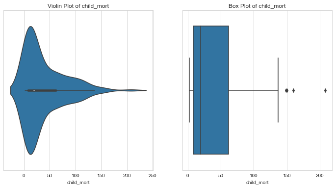
- Notice that half of the countries have a child mortality below 20.
- Further,countries with child mortality less than 1st percentile might not need aid at all. We shall cap their child mortalities to 1st percentile values.
- Countries with extremely high child mortality rate - upper outliers (> 99th percentile) are the perfect candidates for aid. Let’s keep them as they are for further analysis.
1# Removing countries with lower outliers in `child_mort`2countries.loc[l_condition, column] = countries[column].quantile(0.01)
Life Expectancy
1# LIFE EXPECTANCY2column = 'life_expec'3l_condition, u_condition = outlier_analysis(column)
1Quantiles23+------+--------------+4| | life_expec |5|------+--------------|6| 0.1 | 57.82 |7| 0.25 | 65.3 |8| 0.5 | 73.1 |9| 0.75 | 76.8 |10| 0.99 | 82.37 |11+------+--------------+12None131415LOWER OUTLIER THRESHOLD [1st PERCENTILE] FOR life_expec : 47.160000000000004161718Lower Outliers :19+----+-----------+--------------+20| | country | life_expec |21|----+-----------+--------------|22| 66 | Haiti | 32.1 |23| 87 | Lesotho | 46.5 |24+----+-----------+--------------+252627UPPER OUTLIER THRESHOLD [99th PERCENTILE] FOR life_expec : 82.37282930Upper Outliers :31+-----+-----------+--------------+32| | country | life_expec |33|-----+-----------+--------------|34| 133 | Singapore | 82.7 |35| 77 | Japan | 82.8 |36+-----+-----------+--------------+
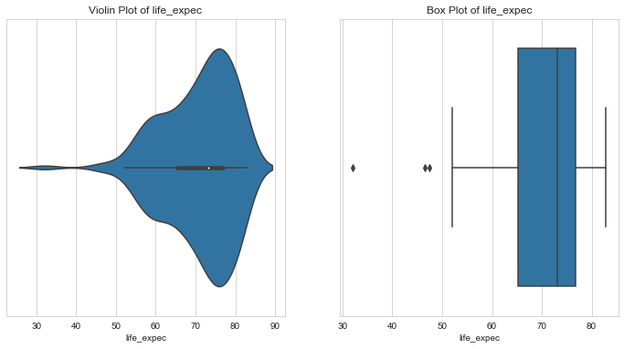
- Some of the lowest life expectancy is seen in Haiti and Lesoto.
- About 50% of the countries have a life expectany of 73 or below and the other 50% have above 73.
- Countries like Singapore and Japan have the highest life expective, better than 99% of the countries.
- Countries with very low life expectancy are possible candidates for aid.
- Hence, let’s keep the lower outliers.
- One the other hand, countries like Singapore and Japan might not need aid but these values would skew our analysis. Let’s cap these outliers.
1# Capping upper outliers in life expectancy2countries.loc[u_condition, column] = countries[column].quantile(0.99)
Fertility
1column = 'total_fer'2l_condition, u_condition = outlier_analysis(column)
1Quantiles23+------+-------------+4| | total_fer |5|------+-------------|6| 0.1 | 1.452 |7| 0.25 | 1.795 |8| 0.5 | 2.41 |9| 0.75 | 3.88 |10| 0.99 | 6.5636 |11+------+-------------+12None131415LOWER OUTLIER THRESHOLD [1st PERCENTILE] FOR total_fer : 1.2431999999999999161718Lower Outliers :19+-----+-------------+-------------+20| | country | total_fer |21|-----+-------------+-------------|22| 133 | Singapore | 1.15 |23| 138 | South Korea | 1.23 |24+-----+-------------+-------------+252627UPPER OUTLIER THRESHOLD [99th PERCENTILE] FOR total_fer : 6.563599999999999282930Upper Outliers :31+-----+-----------+-------------+32| | country | total_fer |33|-----+-----------+-------------|34| 32 | Chad | 6.59 |35| 112 | Niger | 7.49 |36+-----+-----------+-------------+
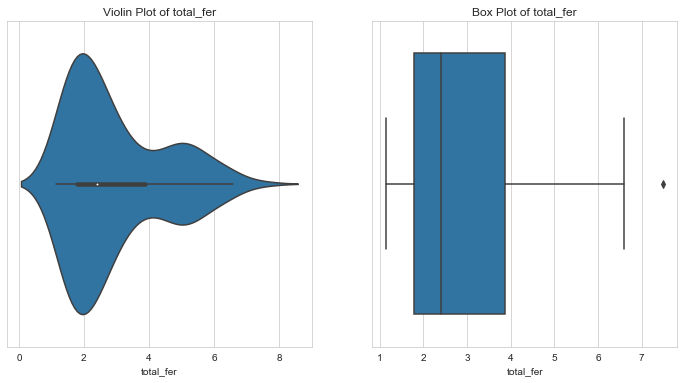
- About 50% of the countries have a fertility of 2.41 or less.
- Lower fertility is seen in developed nations like Singapore and South Korea, where the fertility is less than 99% countries.
- Countries with higher total fertility might need the aid more since this mean more health risk.
- Fertility in Chad and Niger is higher than 99 percent of the countries.
- Since these countries might need the aid, let’s leave these values for further analysis.
- Countries with fertility rates less than 1 perecent of the population look like they are developed nations. Let’s cap these outlier so that they don’t skew our analysis.
- Further, from the violin plot, notice that fertility has two peaks - 2 and 5. This indicates that fertility rate could be used to effectively segregate countries. More analysis is needed here.
1# capping lower outliers in fertility2countries.loc[l_condition,column] = countries[column].quantile(.1)
Health Spending
1# health spending per capita2column = 'health'3l_condition, u_condition = outlier_analysis(column)
1Quantiles23+------+-----------+4| | health |5|------+-----------|6| 0.1 | 36.5026 |7| 0.25 | 78.5355 |8| 0.5 | 321.886 |9| 0.75 | 976.94 |10| 0.99 | 8410.33 |11+------+-----------+12None131415LOWER OUTLIER THRESHOLD [1st PERCENTILE] FOR health : 17.009362000000003161718Lower Outliers :19+----+------------+----------+20| | country | health |21|----+------------+----------|22| 50 | Eritrea | 12.8212 |23| 93 | Madagascar | 15.5701 |24+----+------------+----------+252627UPPER OUTLIER THRESHOLD [99th PERCENTILE] FOR health : 8410.3304282930Upper Outliers :31+-----+---------------+----------+32| | country | health |33|-----+---------------+----------|34| 145 | Switzerland | 8579 |35| 159 | United States | 8663.6 |36+-----+---------------+----------+
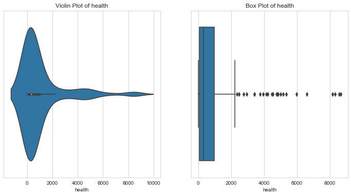
- The countries with more health spending are less in need of aid.
- Like Switzerland and United States, whose health spending is higher than 99% of the countries. But values like these would skew the entire analysis for aid needing countries. Hence, we’d cap these values with the 99th percentile value.
- The countries with less health spending might have variety of reasons like - optimum general health , or bad economic conditions. Let’s keep these values for further analysis.
1# removing upper outliers in health spending2countries.loc[u_condition,column] = countries[column].quantile(0.99)
GDP per capita
1# GDP per capita2column = 'gdpp'3l_condition, u_condition = outlier_analysis(column)
1Quantiles23+------+---------+4| | gdpp |5|------+---------|6| 0.1 | 593.8 |7| 0.25 | 1330 |8| 0.5 | 4660 |9| 0.75 | 14050 |10| 0.99 | 79088 |11+------+---------+12None131415LOWER OUTLIER THRESHOLD [1st PERCENTILE] FOR gdpp : 331.62161718Lower Outliers :19+----+-----------+--------+20| | country | gdpp |21|----+-----------+--------|22| 26 | Burundi | 231 |23| 88 | Liberia | 327 |24+----+-----------+--------+252627UPPER OUTLIER THRESHOLD [99th PERCENTILE] FOR gdpp : 79088.00000000004282930Upper Outliers :31+-----+------------+--------+32| | country | gdpp |33|-----+------------+--------|34| 114 | Norway | 87800 |35| 91 | Luxembourg | 105000 |36+-----+------------+--------+
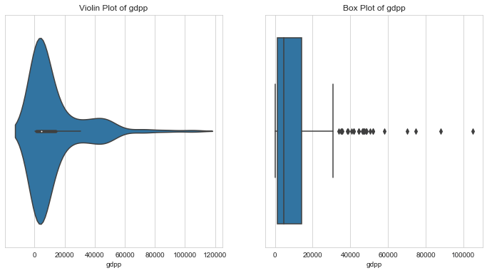
- GDP per capita is a very good indicator of a country’s prosperity
- Notice that there are three peaks in the violin plot of GDP. These might indicate the three clusters - under developed, developing and developed nations.
- Under developed nations are the most in need of aid. Countries like Burundi and Libera have GDPs less than 99% of the countries. Even though they are outliers, let’s keep them for further analysis.
- But, we could cap GDPs which are greater than GDPs of 99% of the countries (Luxembourg & Norway)
1# capping upper outliers in gdpp2countries.loc[u_condition, column] = countries[column].quantile(.99)
Inflation Index
1column = 'inflation'2l_condition, u_condition = outlier_analysis(column)
1Quantiles23+------+-------------+4| | inflation |5|------+-------------|6| 0.1 | 0.5878 |7| 0.25 | 1.81 |8| 0.5 | 5.39 |9| 0.75 | 10.75 |10| 0.99 | 41.478 |11+------+-------------+12None131415LOWER OUTLIER THRESHOLD [1st PERCENTILE] FOR inflation : -2.3487999999999998161718Lower Outliers :19+-----+------------+-------------+20| | country | inflation |21|-----+------------+-------------|22| 131 | Seychelles | -4.21 |23| 73 | Ireland | -3.22 |24+-----+------------+-------------+252627UPPER OUTLIER THRESHOLD [99th PERCENTILE] FOR inflation : 41.47800000000002282930Upper Outliers :31+-----+-----------+-------------+32| | country | inflation |33|-----+-----------+-------------|34| 163 | Venezuela | 45.9 |35| 113 | Nigeria | 104 |36+-----+-----------+-------------+
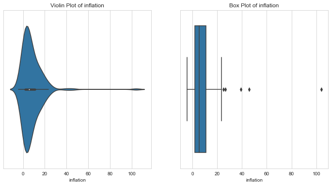
- Very high inflation indicates a bad economic state.
- The violinplot again indicates three peaks - indicating three possible clusters of inflation - each with progressively less countries.
- Countries with very high inflation are might need aid. Since this is our area of interest, let’s keep the upper outliers in inflation as they are for further analysis.
- Let’s cap lower outliers since these look like good economies with no need of aid.
1# capping lower outliers in inflation2countries.loc[l_condition, column] = countries[column].quantile(0.01)
Net Income per person
1# income2column = 'income'3l_condition, u_condition = outlier_analysis(column)
1Quantiles23+------+----------+4| | income |5|------+----------|6| 0.1 | 1524 |7| 0.25 | 3355 |8| 0.5 | 9960 |9| 0.75 | 22800 |10| 0.99 | 84374 |11+------+----------+12None131415LOWER OUTLIER THRESHOLD [1st PERCENTILE] FOR income : 742.24161718Lower Outliers :19+----+------------------+----------+20| | country | income |21|----+------------------+----------|22| 37 | Congo, Dem. Rep. | 609 |23| 88 | Liberia | 700 |24+----+------------------+----------+252627UPPER OUTLIER THRESHOLD [99th PERCENTILE] FOR income : 84374.00000000003282930Upper Outliers :31+-----+------------+----------+32| | country | income |33|-----+------------+----------|34| 91 | Luxembourg | 91700 |35| 123 | Qatar | 125000 |36+-----+------------+----------+
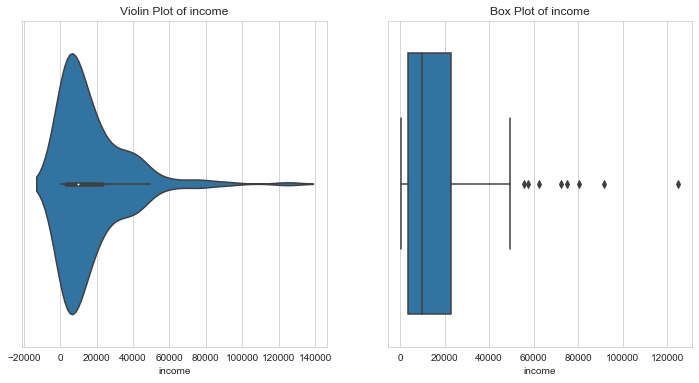
- High net income per person is an indicator of general prosperity of a country. Such countries do not need aid.
- Hence, we shall cap the upper outliers i,e net incomes greater than 99% of that of the other countries.
- Lower outliers, countries with net incomes less than 1% of that of the other countries is our area of interest. Lets leave these values as they are for further analysis.
Imports per capita
1column = 'imports'2l_condition, u_condition = outlier_analysis(column)
1Quantiles23+------+-----------+4| | imports |5|------+-----------|6| 0.1 | 211.006 |7| 0.25 | 640.215 |8| 0.5 | 2045.58 |9| 0.75 | 7719.6 |10| 0.99 | 55371.4 |11+------+-----------+12None131415LOWER OUTLIER THRESHOLD [1st PERCENTILE] FOR imports : 104.90964000000002161718Lower Outliers :19+-----+-----------+-----------+20| | country | imports |21|-----+-----------+-----------|22| 107 | Myanmar | 0.651092 |23| 26 | Burundi | 90.552 |24+-----+-----------+-----------+252627UPPER OUTLIER THRESHOLD [99th PERCENTILE] FOR imports : 55371.39000000013282930Upper Outliers :31+-----+------------+-----------+32| | country | imports |33|-----+------------+-----------|34| 133 | Singapore | 81084 |35| 91 | Luxembourg | 149100 |36+-----+------------+-----------+
Exports per capita
1column = 'exports'2l_condition, u_condition = outlier_analysis(column)
1Quantiles23+------+-----------+4| | exports |5|------+-----------|6| 0.1 | 110.225 |7| 0.25 | 447.14 |8| 0.5 | 1777.44 |9| 0.75 | 7278 |10| 0.99 | 64794.3 |11+------+-----------+12None131415LOWER OUTLIER THRESHOLD [1st PERCENTILE] FOR exports : 22.243716161718Lower Outliers :19+-----+-----------+-----------+20| | country | exports |21|-----+-----------+-----------|22| 107 | Myanmar | 1.07692 |23| 26 | Burundi | 20.6052 |24+-----+-----------+-----------+252627UPPER OUTLIER THRESHOLD [99th PERCENTILE] FOR exports : 64794.26000000014282930Upper Outliers :31+-----+------------+-----------+32| | country | exports |33|-----+------------+-----------|34| 133 | Singapore | 93200 |35| 91 | Luxembourg | 183750 |36+-----+------------+-----------+
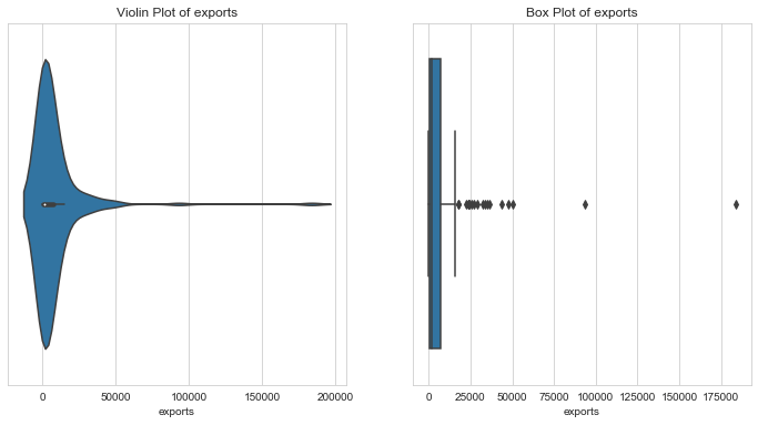
Trade Deficit per capita
1# trade deficit2countries['trade_deficit'] = countries['imports'] - countries['exports']3column = 'trade_deficit'4l_condition, u_condition = outlier_analysis(column)
1Quantiles23+------+-----------------+4| | trade_deficit |5|------+-----------------|6| 0.1 | -3000.82 |7| 0.25 | -327.05 |8| 0.5 | 89.2182 |9| 0.75 | 518.57 |10| 0.99 | 2270.5 |11+------+-----------------+12None131415LOWER OUTLIER THRESHOLD [1st PERCENTILE] FOR trade_deficit : -18426.1161718Lower Outliers :19+-----+------------+-----------------+20| | country | trade_deficit |21|-----+------------+-----------------|22| 91 | Luxembourg | -34650 |23| 123 | Qatar | -27065.5 |24+-----+------------+-----------------+252627UPPER OUTLIER THRESHOLD [99th PERCENTILE] FOR trade_deficit : 2270.500000000002282930Upper Outliers :31+----+-----------+-----------------+32| | country | trade_deficit |33|----+-----------+-----------------|34| 60 | Greece | 2313.4 |35| 10 | Bahamas | 2436 |36+----+-----------+-----------------+
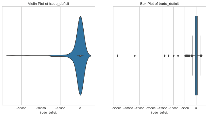
- Trade deficit indicates the balance between exports and imports. Negative trade deficit is favourable indicator of economic health. It means that the country has higher exports compared to imports.
- When the trade deficit is negative, it means that the country is import predominant.
- From the above plot, Greece and Bahamas have a trade deficit higher than 99% of the countries. This could mean a bad economic state. Since this is our key area of interest, we could leave these outliers as they are.
- Countries with negative trade deficit , i.e export predominant countries could be capped to 1st percentile values.
1# capping lower outliers of trade_deficit2countries.loc[l_condition,column] = countries[column].quantile(0.01)
Bivariate Analysis
Pairplot
1# Pair Plots of all variables2sns.pairplot(countries[['child_mort', 'exports', 'health', 'imports', 'income',3 'inflation', 'life_expec', 'total_fer', 'gdpp']]);
1## bivariate analysis boken function2def bivariate_analysis(x_var,y_var,dataframe=countries) :3 # Bivariate Plots with tooltips : country,x,y45 dataframe = dataframe.copy()6 source =ColumnDataSource(dataframe)78 # pallete = ["rgba(38, 70, 83, 1)", 'rgba(42, 157, 143, 1)', "rgba(233, 196, 106, 1)", "rgba(244, 162, 97, 1)", "rgba(231, 111, 81, 1)", '#009cc7']9 pallete = ["#9b59b6", "#3498db", "#95a5a6", "#e74c3c", "#34495e","#38895e",'rgba(42, 157, 143, 1)']1011 # tooltips12 tooltips1 = [13 ("Country", "@country"),14 (x_var,'@'+x_var),15 (y_var,'@'+y_var)16 ]1718 p = figure(plot_width=420, plot_height=400,title='Scatter Plot : '+ x_var+' vs '+y_var, tooltips=tooltips1)1920 p.scatter(x=x_var,y=y_var, fill_alpha=0.6, size=8, source=source, fill_color = "#3498db")21 p.xaxis.axis_label = x_var22 p.yaxis.axis_label = y_var23 reset_output()24 output_notebook()25 show(p)
Child Mortality vs Life Expectancy
1# CHILD MORTALITY vs LIFE EXPECTANCY23x='child_mort'4y = 'life_expec'5bivariate_analysis(x,y)
- looks like
child_mortandlife_expecare almost linearly related. - Life expectancy decreases as child mortality increases.
- One of these features is enough for analysis.
1# Countries with high child mortality and low life expectancy2life_expect_cond = countries['life_expec'] < 603child_mort_cond = countries['child_mort'] > 10045print('Countries with low life expectancy and low Child Mortality Rate')6tab(countries[life_expect_cond & child_mort_cond][['country','child_mort','life_expec']].sort_values(by=['child_mort','life_expec'], ascending=[False,True])[:10])
1Countries with low life expectancy and low Child Mortality Rate2+-----+--------------------------+--------------+--------------+3| | country | child_mort | life_expec |4|-----+--------------------------+--------------+--------------|5| 66 | Haiti | 208 | 32.1 |6| 132 | Sierra Leone | 160 | 55 |7| 32 | Chad | 150 | 56.5 |8| 31 | Central African Republic | 149 | 47.5 |9| 97 | Mali | 137 | 59.5 |10| 112 | Niger | 123 | 58.8 |11| 37 | Congo, Dem. Rep. | 116 | 57.5 |12| 25 | Burkina Faso | 116 | 57.9 |13| 64 | Guinea-Bissau | 114 | 55.6 |14| 40 | Cote d'Ivoire | 111 | 56.3 |15+-----+--------------------------+--------------+--------------+
Child Mortality vs Total Fertility
1# CHILD MORTALITY vs TOTAL FERTILITY23x='child_mort'4y = 'total_fer'5bivariate_analysis(x,y)
1# countries with high fertility and child mortality rate2total_fer_cond = countries['total_fer'] > 63child_mort_cond = countries['child_mort'] > 10045print('Countries with High Total Fertility and Child Mortality Rate')6tab(countries[total_fer_cond & child_mort_cond][['country','total_fer','child_mort']].sort_values(by=['child_mort','total_fer'], ascending=[False,False]))
1Countries with High Total Fertility and Child Mortality Rate2+-----+------------------+-------------+--------------+3| | country | total_fer | child_mort |4|-----+------------------+-------------+--------------|5| 32 | Chad | 6.59 | 150 |6| 97 | Mali | 6.55 | 137 |7| 112 | Niger | 7.49 | 123 |8| 3 | Angola | 6.16 | 119 |9| 37 | Congo, Dem. Rep. | 6.54 | 116 |10+-----+------------------+-------------+--------------+
1# Fertility in countries with extremely high mortality rate2child_mort_cond = countries['child_mort'] > 15034print('Countries with High Total Fertility and Child Mortality Rate')5tab(countries[child_mort_cond][['country','total_fer','child_mort']].sort_values(by=['child_mort','total_fer'], ascending=[False,False]))
1Countries with High Total Fertility and Child Mortality Rate2+-----+--------------+-------------+--------------+3| | country | total_fer | child_mort |4|-----+--------------+-------------+--------------|5| 66 | Haiti | 3.33 | 208 |6| 132 | Sierra Leone | 5.2 | 160 |7+-----+--------------+-------------+--------------+
GDP per capita vs Health Spending
1# GDP per capita vs Health Spending2y='health'3x= 'gdpp'4bivariate_analysis(x,y)
1# Countries with Low GDPP and health spending might need aid2health_cond = countries['health'] < 2003gdpp_cond = countries['gdpp'] < 25004print('Countries with Low GDP and low Health Spending')5tab(countries[health_cond & gdpp_cond][['country','health','gdpp']].sort_values(by=['health','gdpp'], ascending=[True,True])[:10])
1Countries with Low GDP and low Health Spending2+-----+--------------------------+----------+--------+3| | country | health | gdpp |4|-----+--------------------------+----------+--------|5| 50 | Eritrea | 12.8212 | 482 |6| 93 | Madagascar | 15.5701 | 413 |7| 31 | Central African Republic | 17.7508 | 446 |8| 112 | Niger | 17.9568 | 348 |9| 107 | Myanmar | 19.4636 | 988 |10| 106 | Mozambique | 21.8299 | 419 |11| 116 | Pakistan | 22.88 | 1040 |12| 37 | Congo, Dem. Rep. | 26.4194 | 334 |13| 12 | Bangladesh | 26.6816 | 758 |14| 26 | Burundi | 26.796 | 231 |15+-----+--------------------------+----------+--------+
Imports vs GDP per capita
1# IMPORTS vs GDPP2y='imports'3x= 'gdpp'4bivariate_analysis(x,y)
Exports vs GDP per capita
1# Exports vs GDPP2y='exports'3x= 'gdpp'4bivariate_analysis(x,y)
GDP per capita vs Trade Deficit
1y='trade_deficit'2x= 'gdpp'3bivariate_analysis(x,y)
- Trade deficit is a country’s net imports minus exports.
- It indicates the dependence of a country on imports
- Countries with low GDP per capita and positive trade deficit are likely to require aid
- From the above plot, one can see that there are many such countries
1# Countries with positive high trade deficit and low GDP per capita2tr_deficit_cond = countries['trade_deficit'] > 10003gdpp_cond = countries['gdpp'] < 100004print('Countries with high Trade Deficit and Low GDP')5tab(countries[tr_deficit_cond & gdpp_cond][['country','gdpp','trade_deficit']].sort_values(by=['trade_deficit','gdpp'], ascending=[True,False])[:10])
1Countries with high Trade Deficit and Low GDP2+-----+--------------------------------+--------+-----------------+3| | country | gdpp | trade_deficit |4|-----+--------------------------------+--------+-----------------|5| 101 | Micronesia, Fed. Sts. | 2860 | 1644.5 |6| 151 | Tonga | 3550 | 1700.45 |7| 104 | Montenegro | 6680 | 1716.76 |8| 61 | Grenada | 7370 | 1871.98 |9| 141 | St. Vincent and the Grenadines | 6230 | 1881.46 |10| 86 | Lebanon | 8860 | 2161.84 |11+-----+--------------------------------+--------+-----------------+
Net Income per person vs Inflation
1# Income vs Inflation2x = 'inflation'3y = 'income'4bivariate_analysis(x,y)
1# Low Income - High inflation countries might require aid2inflation_cond = countries['inflation'] > 203income_condition = countries['income'] < 100004print('Countries with high inflation and low income')5tab(countries[inflation_cond & income_condition][['country','inflation','income']].sort_values(by=['inflation','income'], ascending=[False, True]))
1Countries with high inflation and low income2+-----+------------------+-------------+----------+3| | country | inflation | income |4|-----+------------------+-------------+----------|5| 113 | Nigeria | 104 | 5150 |6| 103 | Mongolia | 39.2 | 7710 |7| 149 | Timor-Leste | 26.5 | 1850 |8| 165 | Yemen | 23.6 | 4480 |9| 140 | Sri Lanka | 22.8 | 8560 |10| 3 | Angola | 22.4 | 5900 |11| 37 | Congo, Dem. Rep. | 20.8 | 609 |12| 38 | Congo, Rep. | 20.7 | 5190 |13+-----+------------------+-------------+----------+
- Countries with High inflation and low income are possible candidates for aid requirement.
GDP per capita vs Inflation
1x = 'gdpp'2y = 'inflation'3bivariate_analysis(x,y)
- Countries with low GDP percapita and high Inflation are in dire need of support.
- For example, Nigeria has an inflation > 100 while its GDP is 2330.
Correlation Analysis
1plt.figure(figsize=[12,12])2sns.heatmap(countries.corr(),annot=True,cmap='YlGnBu', center=0)
1<matplotlib.axes._subplots.AxesSubplot at 0x7fe87cdf8510>
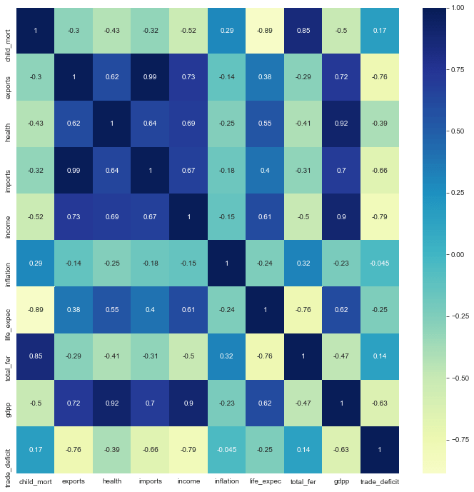
Top Correlations
- Negative Correlation between
life_expecandchild_mort - Positive Correlation between
total_ferandchild_mort
Although clustering analysis is not affected by multicollinearity, this plot shows us the possible linear relationships between different features to help with results obtained from cluster analysis.
Hopkin’s Statistic
1# hopkins test function2from sklearn.neighbors import NearestNeighbors3from random import sample4from numpy.random import uniform5from math import isnan67def hopkins(X):8 d = X.shape[1]9 #d = len(vars) # columns10 n = len(X) # rows11 m = int(0.1 * n)12 nbrs = NearestNeighbors(n_neighbors=1).fit(X.values)1314 rand_X = sample(range(0, n, 1), m)1516 ujd = []17 wjd = []18 for j in range(0, m):19 u_dist, _ = nbrs.kneighbors(uniform(np.amin(X,axis=0),np.amax(X,axis=0),d).reshape(1, -1), 2, return_distance=True)20 ujd.append(u_dist[0][1])21 w_dist, _ = nbrs.kneighbors(X.iloc[rand_X[j]].values.reshape(1, -1), 2, return_distance=True)22 wjd.append(w_dist[0][1])2324 H = sum(ujd) / (sum(ujd) + sum(wjd))25 if isnan(H):26 print(ujd, wjd)27 H = 02829 return H
1## Data used for Clustering2columns_for_clustering = ['child_mort', 'exports', 'health', 'imports', 'income',3 'inflation', 'life_expec', 'total_fer', 'gdpp', 'trade_deficit']4clustering_data = countries[columns_for_clustering].copy()
1# Hopkin's test2n = 103hopkins_statistic = []4for i in range(n) :5 hopkins_statistic.append(hopkins(clustering_data))6print('Min Hopkin\'s Statistic in ',n,'iterations :', min(hopkins_statistic))7print('Max Hopkin\'s Statistic in ',n,'iterations :', max(hopkins_statistic))8print('Mean Hopkin\'s Statistic in ',n,'iterations :', np.mean(hopkins_statistic))9print('Std deviation of Hopkin\'s Statistic in ',n,'iterations :', np.std(hopkins_statistic))
1Min Hopkin's Statistic in 10 iterations : 0.85948517807547232Max Hopkin's Statistic in 10 iterations : 0.97895394407352693Mean Hopkin's Statistic in 10 iterations : 0.94825871725616264Std deviation of Hopkin's Statistic in 10 iterations : 0.03487962411406433
Since hopkin’s statistic is greater than 80% , the data shows good clustering tendency
Standardizing Values
1from sklearn.preprocessing import StandardScaler2scaler = StandardScaler()3clustering_data[columns_for_clustering] = scaler.fit_transform(clustering_data[columns_for_clustering])45tab(clustering_data.describe())
1+-------+---------------+--------------+---------------+---------------+---------------+---------------+--------------+---------------+---------------+-----------------+2| | child_mort | exports | health | imports | income | inflation | life_expec | total_fer | gdpp | trade_deficit |3|-------+---------------+--------------+---------------+---------------+---------------+---------------+--------------+---------------+---------------+-----------------|4| count | 167 | 167 | 167 | 167 | 167 | 167 | 167 | 167 | 167 | 167 |5| mean | -7.97765e-18 | 9.1743e-17 | 2.26033e-17 | 4.65363e-17 | -7.51229e-17 | 8.31005e-17 | 3.7229e-17 | 8.24357e-17 | 8.04413e-17 | 6.18268e-17 |6| std | 1.00301 | 1.00301 | 1.00301 | 1.00301 | 1.00301 | 1.00301 | 1.00301 | 1.00301 | 1.00301 | 1.00301 |7| min | -0.882217 | -0.414037 | -0.583254 | -0.44916 | -0.860326 | -0.964355 | -4.33969 | -1.12962 | -0.720789 | -5.67561 |8| 25% | -0.746668 | -0.389145 | -0.546449 | -0.405554 | -0.717456 | -0.569109 | -0.592657 | -0.767708 | -0.657548 | 0.113986 |9| 50% | -0.47184 | -0.31491 | -0.410154 | -0.309734 | -0.373808 | -0.228871 | 0.287671 | -0.359318 | -0.465925 | 0.247143 |10| 75% | 0.592652 | -0.00795865 | -0.0432751 | 0.0771304 | 0.294237 | 0.280535 | 0.705262 | 0.616834 | 0.0744147 | 0.384486 |11| max | 4.22138 | 9.83981 | 4.11998 | 9.71668 | 5.61154 | 9.14287 | 1.33391 | 3.01405 | 3.81697 | 0.997842 |12+-------+---------------+--------------+---------------+---------------+---------------+---------------+--------------+---------------+---------------+-----------------+
K-Means Clustering
Finding Optimal Number of Clusters
Elbow curve
1# Plotting Elbow curve of Sum of Squared distances of points in each cluster from the centroid of the nearest cluster.2ssd = []3range_n_clusters = np.arange(2,9)4for num_clusters in range_n_clusters :5 kmeans = KMeans(n_clusters=num_clusters)6 kmeans.fit(clustering_data)7 ssd.append(kmeans.inertia_)8plt.plot(range_n_clusters,ssd)9plt.title('Elbow Curve');10plt.xlabel('No of clusters');11plt.ylabel('SSD');
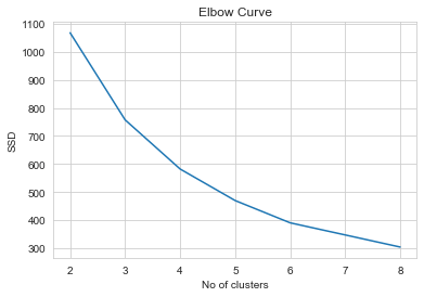
- From the above Elbow curve, one can clearly see that there is a high gradient descent from k=2 to k=4 and then the curve tapers (Change in slope is not as SIGNIFICANT as earlier)
- Hence, k=4 is optimum no of clusters, statistically.
Sihoutte Analysis
1from sklearn.metrics import silhouette_score23no_of_clusters = np.arange(2,10)4score = []56for n_cluster in no_of_clusters :7 kmeans = KMeans(n_clusters=n_cluster, init='k-means++')8 kmeans = kmeans.fit(clustering_data)9 labels = kmeans.labels_10 score.append(silhouette_score(clustering_data,labels))111213plt.title('Silhouette Analysis Plot')14plt.xlabel('No of Clusters')15plt.ylabel('Silhouette Score')16plt.plot(no_of_clusters, score);17print(score)
1[0.46329893684299267, 0.40889975765795494, 0.4113959420115351, 0.40485071262968453, 0.41404360987563693, 0.31039501753497534, 0.302668856614785, 0.30746584335288263]
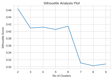
- Higher the silhouette score the better
- However , from the above plot, we see silhouette score is the highest for k = 2, sharply falls at 3 and there’s a local maximum at k=4
- k = 4 seems to be the optimum no of clusters
Final k - Means Clustering
1# k - means clustering algo with k = 42n_cluster = 43kmeans = KMeans(n_clusters=n_cluster, init='k-means++', random_state = 100)4kmeans = kmeans.fit(clustering_data)5labels = kmeans.labels_6countries['k_means_cluster_id'] = labels
1# Countries in each Cluster - k means2for cluster_no in range(n_cluster) :3 condition = countries['k_means_cluster_id'] == cluster_no4 print( 'CLUSTER #',cluster_no,'\n',countries.loc[condition,'country'].values,'\n\n')
1CLUSTER # 02 ['Australia' 'Austria' 'Belgium' 'Brunei' 'Canada' 'Cyprus' 'Denmark'3 'Finland' 'France' 'Germany' 'Greece' 'Iceland' 'Ireland' 'Israel'4 'Italy' 'Japan' 'Kuwait' 'Malta' 'Netherlands' 'New Zealand' 'Norway'5 'Slovenia' 'Spain' 'Sweden' 'Switzerland' 'United Arab Emirates'6 'United Kingdom' 'United States']789CLUSTER # 110 ['Afghanistan' 'Angola' 'Benin' 'Botswana' 'Burkina Faso' 'Burundi'11 'Cameroon' 'Central African Republic' 'Chad' 'Comoros' 'Congo, Dem. Rep.'12 'Congo, Rep.' "Cote d'Ivoire" 'Equatorial Guinea' 'Eritrea' 'Gabon'13 'Gambia' 'Ghana' 'Guinea' 'Guinea-Bissau' 'Haiti' 'Iraq' 'Kenya'14 'Kiribati' 'Lao' 'Lesotho' 'Liberia' 'Madagascar' 'Malawi' 'Mali'15 'Mauritania' 'Mozambique' 'Namibia' 'Niger' 'Nigeria' 'Pakistan' 'Rwanda'16 'Senegal' 'Sierra Leone' 'Solomon Islands' 'South Africa' 'Sudan'17 'Tanzania' 'Timor-Leste' 'Togo' 'Uganda' 'Yemen' 'Zambia']181920CLUSTER # 221 ['Albania' 'Algeria' 'Antigua and Barbuda' 'Argentina' 'Armenia'22 'Azerbaijan' 'Bahamas' 'Bahrain' 'Bangladesh' 'Barbados' 'Belarus'23 'Belize' 'Bhutan' 'Bolivia' 'Bosnia and Herzegovina' 'Brazil' 'Bulgaria'24 'Cambodia' 'Cape Verde' 'Chile' 'China' 'Colombia' 'Costa Rica' 'Croatia'25 'Czech Republic' 'Dominican Republic' 'Ecuador' 'Egypt' 'El Salvador'26 'Estonia' 'Fiji' 'Georgia' 'Grenada' 'Guatemala' 'Guyana' 'Hungary'27 'India' 'Indonesia' 'Iran' 'Jamaica' 'Jordan' 'Kazakhstan'28 'Kyrgyz Republic' 'Latvia' 'Lebanon' 'Libya' 'Lithuania' 'Macedonia, FYR'29 'Malaysia' 'Maldives' 'Mauritius' 'Micronesia, Fed. Sts.' 'Moldova'30 'Mongolia' 'Montenegro' 'Morocco' 'Myanmar' 'Nepal' 'Oman' 'Panama'31 'Paraguay' 'Peru' 'Philippines' 'Poland' 'Portugal' 'Romania' 'Russia'32 'Samoa' 'Saudi Arabia' 'Serbia' 'Seychelles' 'Slovak Republic'33 'South Korea' 'Sri Lanka' 'St. Vincent and the Grenadines' 'Suriname'34 'Tajikistan' 'Thailand' 'Tonga' 'Tunisia' 'Turkey' 'Turkmenistan'35 'Ukraine' 'Uruguay' 'Uzbekistan' 'Vanuatu' 'Venezuela' 'Vietnam']363738CLUSTER # 339 ['Luxembourg' 'Qatar' 'Singapore']
Hierarchical Clustering
HAC : Single Linkage, Euclidean Measure
1# Agglomerative Single Linkage2mergings = linkage(clustering_data,method='single',metric='euclidean')3plt.figure(figsize=[16,10])4plt.title('Single Linkage - Hierarchical Clustering')5dendrogram(mergings);
HAC : Complete Linkage, Euclidean Measure
1# Complete Linkage2mergings = linkage(clustering_data,method='complete',metric='euclidean')3plt.figure(figsize=[16,10])4plt.title('Complete Linkage - Hierarchical Clustering')5dendrogram(mergings);
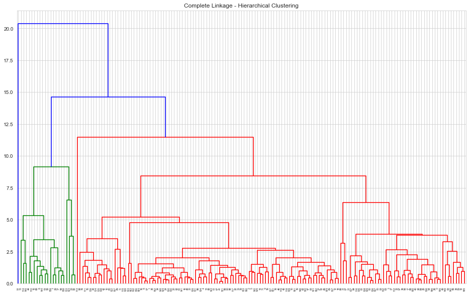
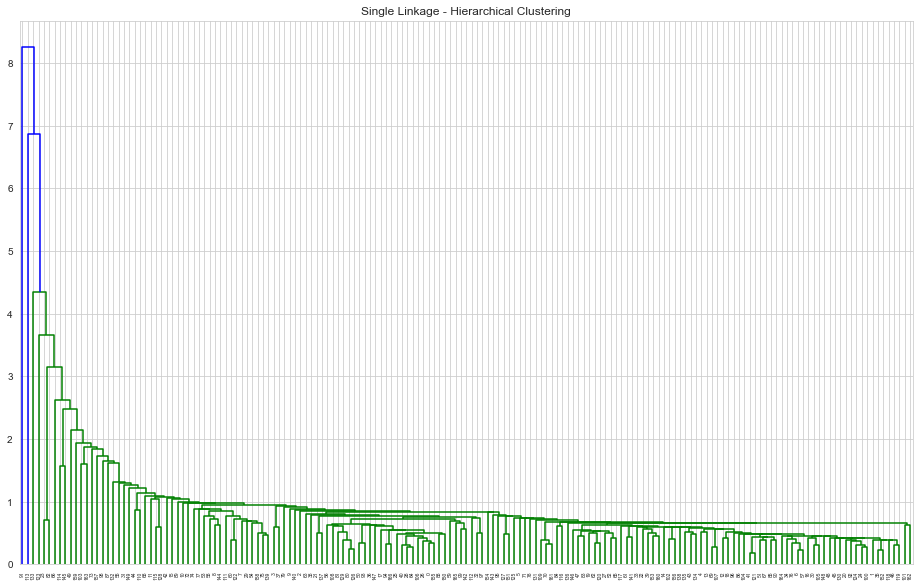
- Hierarchical clustering with complete linkage has a more discriminative dendrogram
1# Using Complete Linkage, cutting the tree for 6 clusters2n_clusters = 63cluster_labels = cut_tree(mergings, n_clusters=n_clusters)4countries['hac_complete_cluster_id'] = cluster_labels
1# Countries in each Cluster - Hierarchical - Complete Linkage2for cluster_no in range(n_clusters) :3 condition = countries['hac_complete_cluster_id'] == cluster_no4 print( 'CLUSTER #',cluster_no,'\n',countries.loc[condition,'country'].values,'\n\n')
1CLUSTER # 02 ['Afghanistan' 'Angola' 'Benin' 'Botswana' 'Burkina Faso' 'Burundi'3 'Cameroon' 'Central African Republic' 'Chad' 'Comoros' 'Congo, Dem. Rep.'4 'Congo, Rep.' "Cote d'Ivoire" 'Equatorial Guinea' 'Eritrea' 'Gabon'5 'Gambia' 'Ghana' 'Guinea' 'Guinea-Bissau' 'Haiti' 'Iraq' 'Kenya'6 'Kiribati' 'Lao' 'Lesotho' 'Liberia' 'Madagascar' 'Malawi' 'Mali'7 'Mauritania' 'Mozambique' 'Namibia' 'Niger' 'Pakistan' 'Rwanda' 'Senegal'8 'Sierra Leone' 'Solomon Islands' 'South Africa' 'Sudan' 'Tanzania'9 'Timor-Leste' 'Togo' 'Uganda' 'Yemen' 'Zambia']101112CLUSTER # 113 ['Albania' 'Algeria' 'Antigua and Barbuda' 'Argentina' 'Armenia'14 'Azerbaijan' 'Bahamas' 'Bahrain' 'Bangladesh' 'Barbados' 'Belarus'15 'Belize' 'Bhutan' 'Bolivia' 'Bosnia and Herzegovina' 'Brazil' 'Bulgaria'16 'Cambodia' 'Cape Verde' 'Chile' 'China' 'Colombia' 'Costa Rica' 'Croatia'17 'Cyprus' 'Czech Republic' 'Dominican Republic' 'Ecuador' 'Egypt'18 'El Salvador' 'Estonia' 'Fiji' 'Georgia' 'Greece' 'Grenada' 'Guatemala'19 'Guyana' 'Hungary' 'India' 'Indonesia' 'Iran' 'Israel' 'Italy' 'Jamaica'20 'Jordan' 'Kazakhstan' 'Kyrgyz Republic' 'Latvia' 'Lebanon' 'Libya'21 'Lithuania' 'Macedonia, FYR' 'Malaysia' 'Maldives' 'Malta' 'Mauritius'22 'Micronesia, Fed. Sts.' 'Moldova' 'Mongolia' 'Montenegro' 'Morocco'23 'Myanmar' 'Nepal' 'New Zealand' 'Oman' 'Panama' 'Paraguay' 'Peru'24 'Philippines' 'Poland' 'Portugal' 'Romania' 'Russia' 'Samoa'25 'Saudi Arabia' 'Serbia' 'Seychelles' 'Slovak Republic' 'Slovenia'26 'South Korea' 'Spain' 'Sri Lanka' 'St. Vincent and the Grenadines'27 'Suriname' 'Tajikistan' 'Thailand' 'Tonga' 'Tunisia' 'Turkey'28 'Turkmenistan' 'Ukraine' 'United Arab Emirates' 'Uruguay' 'Uzbekistan'29 'Vanuatu' 'Venezuela' 'Vietnam']303132CLUSTER # 233 ['Australia' 'Austria' 'Belgium' 'Canada' 'Denmark' 'Finland' 'France'34 'Germany' 'Iceland' 'Ireland' 'Japan' 'Netherlands' 'Norway' 'Sweden'35 'Switzerland' 'United Kingdom' 'United States']363738CLUSTER # 339 ['Brunei' 'Kuwait' 'Qatar' 'Singapore']404142CLUSTER # 443 ['Luxembourg']444546CLUSTER # 547 ['Nigeria']
HAC : Average Linkage, Euclidean Measure
1# Average Linkage2mergings = linkage(clustering_data,method='average',metric='euclidean')3plt.figure(figsize=[16,10])4plt.title('Average Linkage - Hierarchical Clustering')5dendrogram(mergings);
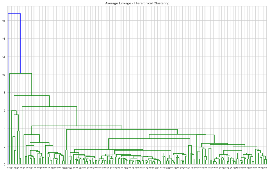
1# Using Average Linkage, cutting the tree for 6 clusters2n_clusters = 63cluster_labels = cut_tree(mergings, n_clusters=n_clusters)4countries['hac_average_cluster_id'] = cluster_labels
1# Countries in each Cluster - Hierarchical - average Linkage2for cluster_no in range(n_clusters) :3 condition = countries['hac_average_cluster_id'] == cluster_no4 print( 'CLUSTER #',cluster_no,'\n',countries.loc[condition,'country'].values,'\n\n')
1CLUSTER # 02 ['Afghanistan' 'Albania' 'Algeria' 'Angola' 'Antigua and Barbuda'3 'Argentina' 'Armenia' 'Australia' 'Austria' 'Azerbaijan' 'Bahamas'4 'Bahrain' 'Bangladesh' 'Barbados' 'Belarus' 'Belgium' 'Belize' 'Benin'5 'Bhutan' 'Bolivia' 'Bosnia and Herzegovina' 'Botswana' 'Brazil'6 'Bulgaria' 'Burkina Faso' 'Burundi' 'Cambodia' 'Cameroon' 'Canada'7 'Cape Verde' 'Central African Republic' 'Chad' 'Chile' 'China' 'Colombia'8 'Comoros' 'Congo, Dem. Rep.' 'Congo, Rep.' 'Costa Rica' "Cote d'Ivoire"9 'Croatia' 'Cyprus' 'Czech Republic' 'Denmark' 'Dominican Republic'10 'Ecuador' 'Egypt' 'El Salvador' 'Equatorial Guinea' 'Eritrea' 'Estonia'11 'Fiji' 'Finland' 'France' 'Gabon' 'Gambia' 'Georgia' 'Germany' 'Ghana'12 'Greece' 'Grenada' 'Guatemala' 'Guinea' 'Guinea-Bissau' 'Guyana'13 'Hungary' 'Iceland' 'India' 'Indonesia' 'Iran' 'Iraq' 'Israel' 'Italy'14 'Jamaica' 'Japan' 'Jordan' 'Kazakhstan' 'Kenya' 'Kiribati'15 'Kyrgyz Republic' 'Lao' 'Latvia' 'Lebanon' 'Lesotho' 'Liberia' 'Libya'16 'Lithuania' 'Macedonia, FYR' 'Madagascar' 'Malawi' 'Malaysia' 'Maldives'17 'Mali' 'Malta' 'Mauritania' 'Mauritius' 'Micronesia, Fed. Sts.' 'Moldova'18 'Mongolia' 'Montenegro' 'Morocco' 'Mozambique' 'Myanmar' 'Namibia'19 'Nepal' 'Netherlands' 'New Zealand' 'Niger' 'Oman' 'Pakistan' 'Panama'20 'Paraguay' 'Peru' 'Philippines' 'Poland' 'Portugal' 'Romania' 'Russia'21 'Rwanda' 'Samoa' 'Saudi Arabia' 'Senegal' 'Serbia' 'Seychelles'22 'Sierra Leone' 'Slovak Republic' 'Slovenia' 'Solomon Islands'23 'South Africa' 'South Korea' 'Spain' 'Sri Lanka'24 'St. Vincent and the Grenadines' 'Sudan' 'Suriname' 'Sweden' 'Tajikistan'25 'Tanzania' 'Thailand' 'Timor-Leste' 'Togo' 'Tonga' 'Tunisia' 'Turkey'26 'Turkmenistan' 'Uganda' 'Ukraine' 'United Arab Emirates' 'United Kingdom'27 'United States' 'Uruguay' 'Uzbekistan' 'Vanuatu' 'Venezuela' 'Vietnam'28 'Yemen' 'Zambia']293031CLUSTER # 132 ['Brunei' 'Ireland' 'Kuwait' 'Norway' 'Qatar' 'Switzerland']333435CLUSTER # 236 ['Haiti']373839CLUSTER # 340 ['Luxembourg']414243CLUSTER # 444 ['Nigeria']454647CLUSTER # 548 ['Singapore']
HAC : Complete Linkage , Correlation Measure
1## HAC Clustering : Dissimilarity Measure : Correlation2hac_correlation_mergings = linkage(clustering_data,method='complete', metric='correlation')3plt.figure(figsize=[12,12])4plt.title('Hierarchical Clustering : Complete Linkage, Correlation Measure')5dendrogram(hac_correlation_mergings);
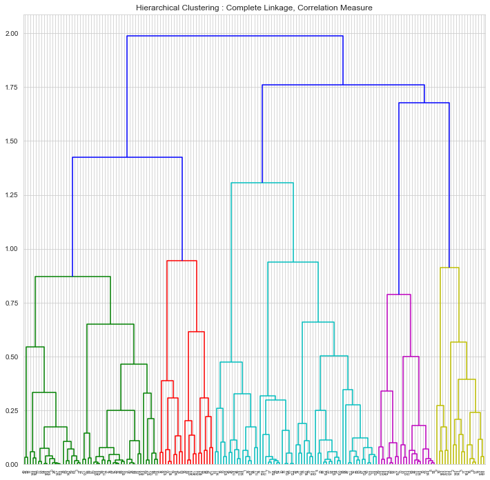
1n_clusters = 62labels = cut_tree(hac_correlation_mergings, n_clusters=n_clusters)3countries['hac_correlation_cluster_id'] = labels
1# HAC clustering : Correlation measure : complete distance : Countries in each cluster23for cluster_no in range(n_clusters) :4 condition = countries['hac_correlation_cluster_id'] == cluster_no5 print( 'CLUSTER #',cluster_no,'\n',countries.loc[condition,'country'].values,'\n\n')
1CLUSTER # 02 ['Afghanistan' 'Angola' 'Benin' 'Botswana' 'Burkina Faso' 'Burundi'3 'Cameroon' 'Central African Republic' 'Chad' 'Comoros' 'Congo, Dem. Rep.'4 'Congo, Rep.' "Cote d'Ivoire" 'Equatorial Guinea' 'Eritrea' 'Gabon'5 'Gambia' 'Ghana' 'Guinea' 'Guinea-Bissau' 'Haiti' 'India' 'Iraq' 'Kenya'6 'Kiribati' 'Lao' 'Lesotho' 'Liberia' 'Madagascar' 'Malawi' 'Mali'7 'Mauritania' 'Mozambique' 'Myanmar' 'Namibia' 'Niger' 'Pakistan' 'Rwanda'8 'Senegal' 'Sierra Leone' 'South Africa' 'Sudan' 'Tanzania' 'Timor-Leste'9 'Togo' 'Turkmenistan' 'Uganda' 'Yemen' 'Zambia']101112CLUSTER # 113 ['Albania' 'Belize' 'Cape Verde' 'Colombia' 'Dominican Republic' 'Ecuador'14 'El Salvador' 'Grenada' 'Maldives' 'Morocco' 'Panama' 'Paraguay' 'Peru'15 'St. Vincent and the Grenadines' 'Thailand' 'Tunisia']161718CLUSTER # 219 ['Algeria' 'Argentina' 'Armenia' 'Azerbaijan' 'Belarus' 'Georgia' 'Iran'20 'Jamaica' 'Kazakhstan' 'Moldova' 'Mongolia' 'Nigeria' 'Russia'21 'Sri Lanka' 'Suriname' 'Ukraine' 'Venezuela' 'Vietnam']222324CLUSTER # 325 ['Antigua and Barbuda' 'Australia' 'Bahamas' 'Barbados'26 'Bosnia and Herzegovina' 'Brazil' 'Bulgaria' 'Canada' 'Chile' 'China'27 'Costa Rica' 'Croatia' 'Cyprus' 'Czech Republic' 'Estonia' 'France'28 'Greece' 'Hungary' 'Israel' 'Italy' 'Japan' 'Latvia' 'Lebanon'29 'Lithuania' 'Macedonia, FYR' 'Malaysia' 'Malta' 'Mauritius' 'Montenegro'30 'New Zealand' 'Poland' 'Portugal' 'Romania' 'Serbia' 'Seychelles'31 'Slovak Republic' 'Slovenia' 'South Korea' 'Spain' 'Turkey'32 'United Kingdom' 'United States' 'Uruguay']333435CLUSTER # 436 ['Austria' 'Bahrain' 'Belgium' 'Brunei' 'Denmark' 'Finland' 'Germany'37 'Iceland' 'Ireland' 'Kuwait' 'Libya' 'Luxembourg' 'Netherlands' 'Norway'38 'Oman' 'Qatar' 'Saudi Arabia' 'Singapore' 'Sweden' 'Switzerland'39 'United Arab Emirates']404142CLUSTER # 543 ['Bangladesh' 'Bhutan' 'Bolivia' 'Cambodia' 'Egypt' 'Fiji' 'Guatemala'44 'Guyana' 'Indonesia' 'Jordan' 'Kyrgyz Republic' 'Micronesia, Fed. Sts.'45 'Nepal' 'Philippines' 'Samoa' 'Solomon Islands' 'Tajikistan' 'Tonga'46 'Uzbekistan' 'Vanuatu']
Mixed K-Means Clustering
1# Performing k-means using results of Hierarchical clustering2# 1. No of clusters of Hierarchical Clustering3# 2. Centroids obtainded from Hierarchical Clustering as the initialization points.4clustering_data['k_means_cluster_id'] = countries['k_means_cluster_id']5clustering_data['hac_correlation_cluster_id'] = countries['hac_correlation_cluster_id']6columns = columns_for_clustering.copy()7columns.extend(['hac_correlation_cluster_id'])8centroids = clustering_data[columns].groupby(['hac_correlation_cluster_id']).mean()9n_clusters = 610mixed_kmeans = KMeans(n_clusters=6 , init = centroids.values, random_state=100)11results = mixed_kmeans.fit(clustering_data[columns_for_clustering])
1countries['mixed_cluster_id'] = results.labels_
1# Mixed clustering : Euclidean measure : k-means : Countries in each cluster23for cluster_no in range(n_clusters) :4 condition = countries['mixed_cluster_id'] == cluster_no5 print( 'CLUSTER #',cluster_no,'\n',countries.loc[condition,'country'].values,'\n\n')
1CLUSTER # 02 ['Afghanistan' 'Angola' 'Benin' 'Burkina Faso' 'Burundi' 'Cameroon'3 'Central African Republic' 'Chad' 'Comoros' 'Congo, Dem. Rep.'4 'Congo, Rep.' "Cote d'Ivoire" 'Equatorial Guinea' 'Gambia' 'Guinea'5 'Guinea-Bissau' 'Haiti' 'Lesotho' 'Liberia' 'Malawi' 'Mali' 'Mauritania'6 'Mozambique' 'Niger' 'Sierra Leone' 'Sudan' 'Tanzania' 'Timor-Leste'7 'Togo' 'Uganda' 'Zambia']8910CLUSTER # 111 ['Albania' 'Algeria' 'Antigua and Barbuda' 'Argentina' 'Armenia'12 'Azerbaijan' 'Bahrain' 'Barbados' 'Belarus' 'Belize'13 'Bosnia and Herzegovina' 'Brazil' 'Bulgaria' 'Cape Verde' 'Chile' 'China'14 'Colombia' 'Costa Rica' 'Croatia' 'Czech Republic' 'Dominican Republic'15 'Ecuador' 'El Salvador' 'Estonia' 'Georgia' 'Grenada' 'Hungary' 'Iran'16 'Jamaica' 'Jordan' 'Kazakhstan' 'Latvia' 'Lebanon' 'Libya' 'Lithuania'17 'Macedonia, FYR' 'Malaysia' 'Maldives' 'Mauritius' 'Moldova' 'Montenegro'18 'Morocco' 'Oman' 'Panama' 'Paraguay' 'Peru' 'Poland' 'Romania' 'Russia'19 'Saudi Arabia' 'Serbia' 'Seychelles' 'Slovak Republic' 'South Korea'20 'Sri Lanka' 'St. Vincent and the Grenadines' 'Suriname' 'Thailand'21 'Tunisia' 'Turkey' 'Ukraine' 'Uruguay' 'Vietnam']222324CLUSTER # 225 ['Mongolia' 'Nigeria' 'Venezuela']262728CLUSTER # 329 ['Australia' 'Austria' 'Bahamas' 'Belgium' 'Canada' 'Cyprus' 'Denmark'30 'Finland' 'France' 'Germany' 'Greece' 'Iceland' 'Israel' 'Italy' 'Japan'31 'Malta' 'Netherlands' 'New Zealand' 'Portugal' 'Slovenia' 'Spain'32 'Sweden' 'United Arab Emirates' 'United Kingdom' 'United States']333435CLUSTER # 436 ['Brunei' 'Ireland' 'Kuwait' 'Luxembourg' 'Norway' 'Qatar' 'Singapore'37 'Switzerland']383940CLUSTER # 541 ['Bangladesh' 'Bhutan' 'Bolivia' 'Botswana' 'Cambodia' 'Egypt' 'Eritrea'42 'Fiji' 'Gabon' 'Ghana' 'Guatemala' 'Guyana' 'India' 'Indonesia' 'Iraq'43 'Kenya' 'Kiribati' 'Kyrgyz Republic' 'Lao' 'Madagascar'44 'Micronesia, Fed. Sts.' 'Myanmar' 'Namibia' 'Nepal' 'Pakistan'45 'Philippines' 'Rwanda' 'Samoa' 'Senegal' 'Solomon Islands' 'South Africa'46 'Tajikistan' 'Tonga' 'Turkmenistan' 'Uzbekistan' 'Vanuatu' 'Yemen']
1# silhouette scores of all the methods2print('Mixed Clustering',silhouette_score(clustering_data[columns_for_clustering],countries['mixed_cluster_id']))3print('K-means Clustering',silhouette_score(clustering_data[columns_for_clustering],countries['k_means_cluster_id']))4print('Hierarchical Correlation Clustering',silhouette_score(clustering_data[columns_for_clustering],countries['hac_correlation_cluster_id']))
1Mixed Clustering 0.2950259022612962K-means Clustering 0.41139594201153513Hierarchical Correlation Clustering 0.06816978634185641
Cluster Profiling
1# Clustering Profling - Plots using Bokeh23cluster_id_column = 'hierarchical-c-link-cluster-id'4title="Hierarchical Clustering"56def cluster_analysis_plot(cluster_id_column,title,x_var='income',y_var='child_mort',z_var='gdpp',dataframe=countries) :7 # Plots8 # works upto 6 clusters910 dataframe = dataframe.copy()11 dataframe[cluster_id_column] = dataframe[cluster_id_column].astype('str')12 source =ColumnDataSource(dataframe)1314 cluster_ids = sorted(dataframe[cluster_id_column].unique())1516 # pallete = ["rgba(38, 70, 83, 1)", 'rgba(42, 157, 143, 1)', "rgba(233, 196, 106, 1)", "rgba(244, 162, 97, 1)", "rgba(231, 111, 81, 1)", '#009cc7']17 pallete = ["#9b59b6", "#3498db", "#95a5a6", "#e74c3c", "#34495e","#38895e",'rgba(42, 157, 143, 1)']1819 mapper = factor_cmap(cluster_id_column,palette=pallete[:len(cluster_ids)], factors = cluster_ids)2021 # plot 122 tooltips1 = [23 ("Country", "@country"),24 (z_var,'@'+z_var),25 (x_var,'@'+x_var),26 ('Cluster', '@'+cluster_id_column)27 ]2829 p = figure(plot_width=420, plot_height=400,title=title+ ' : '+ z_var+' vs '+x_var, tooltips=tooltips1, toolbar_location=None)30 for num,index in enumerate(cluster_ids) :31 condition = dataframe[cluster_id_column] == index32 source = dataframe[condition]33 p.scatter(x=z_var,y=x_var, fill_alpha=0.6, size=8, source=source, fill_color = pallete[num] , muted_alpha=0.1, legend_label=index)34 p.xaxis.axis_label = z_var35 p.yaxis.axis_label = x_var36 p.legend.click_policy="mute"37 # ----------------------------38 #Plot 23940 tooltips2 = [41 ("Country", "@country"),42 (z_var,'@'+z_var),43 (y_var,'@'+y_var),44 ('Cluster', '@'+cluster_id_column)45 ]464748 q = figure(plot_width=420, plot_height=400,title=title+ ' : '+ z_var+' vs '+y_var, tooltips=tooltips2, toolbar_location=None)4950 for num,index in enumerate(cluster_ids) :51 condition = dataframe[cluster_id_column] == index52 source = dataframe[condition]53 q.scatter(x=z_var,y=y_var, fill_alpha=0.6, size=8, source=source, fill_color = pallete[num] , muted_alpha=0.1, legend_label=index)54 q.xaxis.axis_label = z_var55 q.yaxis.axis_label = y_var56 q.legend.click_policy="mute"5758 # ----------------------------59 #Plot 36061 tooltips3 = [62 ("Country", "@country"),63 (x_var,'@'+x_var),64 (y_var,'@'+y_var),65 ('Cluster', '@'+cluster_id_column)66 ]6768 r = figure(plot_width=420, plot_height=400,title=title+ ' : '+ x_var+' vs '+y_var, tooltips=tooltips3, toolbar_location=None)6970 for num,index in enumerate(cluster_ids) :71 condition = dataframe[cluster_id_column] == index72 source = dataframe[condition]73 r.scatter(x=x_var,y=y_var, fill_alpha=0.6, size=8, source=source, fill_color = pallete[num] , legend_label=index, muted_alpha=0.1 )7475 r.xaxis.axis_label = x_var76 r.yaxis.axis_label = y_var77 r.legend.click_policy="mute"787980 show(row(p,q,r))
K-Means
1# Cluster Profiling for k-means with 4 clusters2# hover for country names and x, y values , cluster no3# Click on legend to selectively view clusters4cluster_analysis_plot('k_means_cluster_id','k-means clusters')
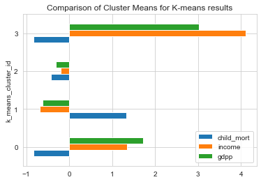
1# Comparing k-means Clusters using mean values of features2clustering_data[['child_mort','income','gdpp','k_means_cluster_id']].groupby('k_means_cluster_id').mean().plot(kind='barh')3plt.title('Comparison of Cluster Means for K-means results');
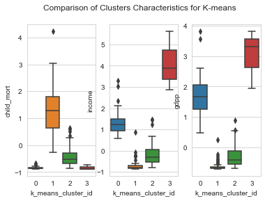
1plot_columns = ['child_mort','income','gdpp']23for idx,column in enumerate(plot_columns) :4 plt.suptitle('Comparison of Clusters Characteristics for K-means');5 plt.subplot('13'+str(idx+1))6 sns.boxplot(y=column, x='k_means_cluster_id',data=clustering_data)
1plt.figure(figsize=[8,8])2pd.plotting.parallel_coordinates(clustering_data, 'k_means_cluster_id', color=["#9b59b6", "#3498db", "#95a5a6", "#e74c3c", "#34495e"]);3plt.title('Parallel Coordinate Plot for K-means')4plt.xticks(rotation=45);
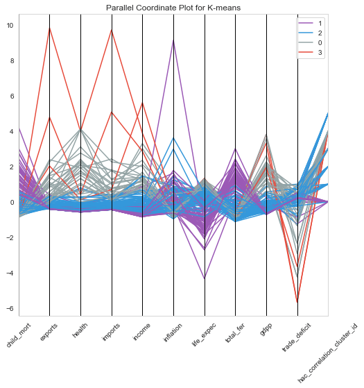
From the above plots, we could characterize features of each cluster as within the following levels.
- Levels : Low, Moderate, High , very high
Characteristics of each cluster
| Cluster | GDP | Income | Child Mortality |
| 0 | High | High to Very High | Low |
| 1 | Low | Low | High to Very High |
| 2 | Low to Moderate | Low to Moderate | Low to Moderate |
| 3 | Very High | Very High | Low |
From the characteristics , we see that the Cluster 1 is our area of interest. Lets look at the countries in Cluster 1.
1# Countries in cluster with area of interest2condition = countries['k_means_cluster_id'] == 13countries.loc[condition,['country','child_mort','income','gdpp']].sort_values(by=['child_mort','income','gdpp'], ascending=[False,True,True])[:5]
| country | child_mort | income | gdpp | |
| 66 | Haiti | 208.0 | 1500 | 662.0 |
| 132 | Sierra Leone | 160.0 | 1220 | 399.0 |
| 32 | Chad | 150.0 | 1930 | 897.0 |
| 31 | Central African Republic | 149.0 | 888 | 446.0 |
| 97 | Mali | 137.0 | 1870 | 708.0 |
Hierarchical Clustering - Complete Linkage, Correlation based distance
1# HAC : Complete linkage, Correlation based distance : cluster analysis plot2# hover for country names and x, y values , cluster no3# Click on legend to selectively view clusters4cluster_analysis_plot('hac_correlation_cluster_id','HAC CORRELATION CLUSTERS')
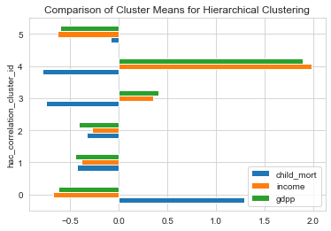
1# Comparing Hierarchical Clusters using mean values of features2clustering_data['hac_correlation_cluster_id'] = countries['hac_correlation_cluster_id']3clustering_data[['child_mort','income','gdpp','hac_correlation_cluster_id']].groupby('hac_correlation_cluster_id').mean().plot(kind='barh');4plt.title('Comparison of Cluster Means for Hierarchical Clustering');
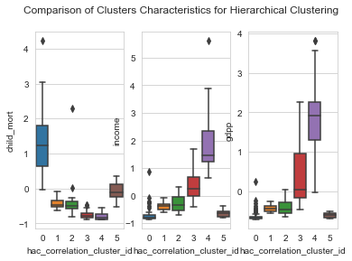
1# box plots2plot_columns = ['child_mort','income','gdpp']34for idx,column in enumerate(plot_columns) :5 plt.suptitle('Comparison of Clusters Characteristics for Hierarchical Clustering');6 plt.subplot('13'+str(idx+1))7 sns.boxplot(y=column, x='hac_correlation_cluster_id',data=clustering_data)
1# Parallel Coordinates plot for Hierarchical clustering with correlation measure and complet linkage2plt.figure(figsize=[8,8])3pd.plotting.parallel_coordinates(clustering_data, 'hac_correlation_cluster_id', color=["#9b59b6", "#3498db", "#95a5a6", "#e74c3c", "#34495e","#38895e",'rgba(42, 157, 143, 1)']);4plt.title('Parallel Coordinate Plot for HAC with Correlation Measure and Complete Linkage')5plt.xticks(rotation=45);
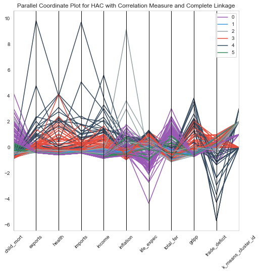
From the above plots, we could characterize features of each cluster as within the following levels.
- Levels : Very low , low, Moderate, High , very high
Characteristics of each cluster
| Cluster | GDP | Income | Child Mortality |
| 0 | Very low | Very Low | Very High |
| 1 | low | low | low |
| 2 | Moderate | Moderate | Moderate |
| 3 | High | High | Low |
| 4 | Very High | Very High | Low |
| 5 | Very Low | Very Low | Low |
From the characteristics , we see that the Cluster 0 is our area of interest. Lets look at the countries in Cluster 0.
1# Countries in cluster with area of interest2condition = countries['hac_correlation_cluster_id'] == 03countries.loc[condition,['country','child_mort','income','gdpp']].sort_values(by=['child_mort','income','gdpp'], ascending=[False,True,True])[:5]
| country | child_mort | income | gdpp | |
| 66 | Haiti | 208.0 | 1500 | 662.0 |
| 132 | Sierra Leone | 160.0 | 1220 | 399.0 |
| 32 | Chad | 150.0 | 1930 | 897.0 |
| 31 | Central African Republic | 149.0 | 888 | 446.0 |
| 97 | Mali | 137.0 | 1870 | 708.0 |
Mixed Clustering : K-means initialized with Hierarchical Cluster Centroids
1cluster_analysis_plot('mixed_cluster_id','MIXED K-MEANS CLUSTERS')
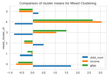
1# Comparing MIXED k-means Clusters using mean values of features2clustering_data['mixed_cluster_id'] = countries['mixed_cluster_id']3clustering_data[['child_mort','income','gdpp','mixed_cluster_id']].groupby('mixed_cluster_id').mean().plot(kind='barh')4plt.title('Comparison of cluster means for Mixed Clustering');
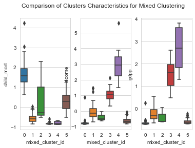
1# box plots2plot_columns = ['child_mort','income','gdpp']34for idx,column in enumerate(plot_columns) :5 plt.suptitle('Comparison of Clusters Characteristics for Mixed Clustering');6 plt.subplot('13'+str(idx+1))7 sns.boxplot(y=column, x='mixed_cluster_id',data=clustering_data)
1# parallel coordinate plot2plt.figure(figsize=[8,8])3pd.plotting.parallel_coordinates(clustering_data, 'mixed_cluster_id', color=["#9b59b6", "#3498db", "#95a5a6", "#e74c3c", "#34495e","#38895e",'rgba(42, 157, 143, 1)']);4plt.title('Parallel Coordinate Plot for Mixed Clustering');5plt.xticks(rotation=45);
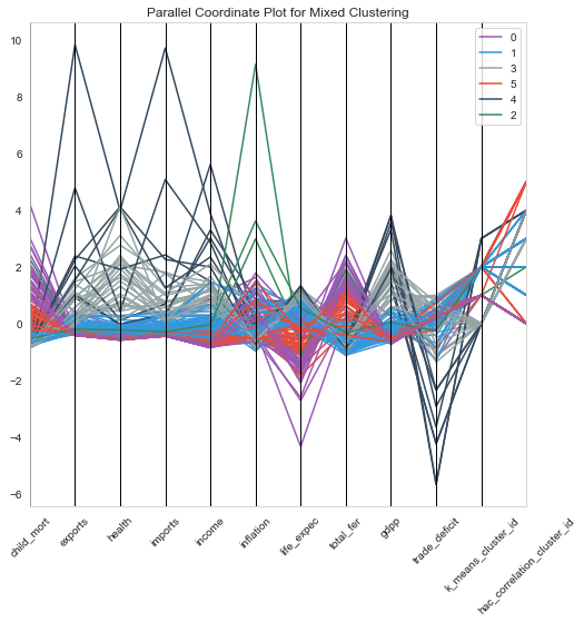
- From the above plots, Cluster 0 has the very low income and gdpp and very high child mortality. Hence, Cluster 0 is the area of interest.
1# Countries in cluster with area of interest2condition = countries['mixed_cluster_id'] == 03countries.loc[condition,['country','child_mort','income','gdpp']].sort_values(by=['child_mort','income','gdpp'], ascending=[False,True,True])[:5]
| country | child_mort | income | gdpp | |
| 66 | Haiti | 208.0 | 1500 | 662.0 |
| 132 | Sierra Leone | 160.0 | 1220 | 399.0 |
| 32 | Chad | 150.0 | 1930 | 897.0 |
| 31 | Central African Republic | 149.0 | 888 | 446.0 |
| 97 | Mali | 137.0 | 1870 | 708.0 |
- Hence , the top five countries to extend aid are
- Haiti
- Sierra Leone
- Chad
- Central African Republic
- Mali
Conclusion
Columns : ‘child_mort’, ‘exports’, ‘health’, ‘imports’, ‘income’,‘inflation’, ‘life_expec’, ‘total_fer’, ‘gdpp’,‘trade_deficit’ were used for clustering.
Hopkin’s Statistic was calculated which showed a very high mean clustering tendency of 96% with a standard deviation of 4%
The dataset was standardized with mean = 0 , standard deviation = 1 before clustering.
Optimum no of clusters for k-means was found to be 4 , both from Elbow curve and Silhoeutte Analysis curve.
Clustering with k-means was performed (Cluster centers initialized with k-means++)
Hierarchical Clustering with Single, Complete and Average linkages and Euclidean , correlation based distances were explored.
Mixed k-means clustering - K-means initialized with centroids of hierarchical clustering - was also explored.
Due to more interpretable results, Hierarchical Clustering with Complete linkage and correlation based distance measure was chosen to arrive at the results.
Characteristics of Clusters obtained :
| Cluster | GDP | Income | Child Mortality |
| 0 | Very low | Very Low | Very High |
| 1 | low | low | low |
| 2 | Moderate | Moderate | Moderate |
| 3 | High | High | Low |
| 4 | Very High | Very High | Low |
| 5 | Very Low | Very Low | Low |
- From the characteristics , we see that the Cluster 0 is our area of interest.
- According to the UN goals of 2030, the top priority is health and then poverty.
- Hence countries in cluster 0 were ranked based on Child Mortality followed by income and GDP per capita.
- By that criteria, the following are the five countries HELP should consider extending their aid.
- Haiti
- Sierra Leone
- Chad
- Central African Republic
- Mali