Boom Bikes Demand Analysis

Problem Statement

A bike-sharing system is a service in which bikes are made available for shared use to individuals on a short term basis for a price or free. Many bike share systems allow people to borrow a bike from a “dock” which is usually computer-controlled wherein the user enters the payment information, and the system unlocks it. This bike can then be returned to another dock belonging to the same system.

A US bike-sharing provider BoomBikes has recently suffered considerable dips in their revenues due to the ongoing Corona pandemic. The company is finding it very difficult to sustain in the current market scenario. So, it has decided to come up with a mindful business plan to be able to accelerate its revenue as soon as the ongoing lockdown comes to an end, and the economy restores to a healthy state.

In such an attempt, BoomBikes aspires to understand the demand for shared bikes among the people after this ongoing quarantine situation ends across the nation due to Covid-19. They have planned this to prepare themselves to cater to the people’s needs once the situation gets better all around and stand out from other service providers and make huge profits.

They have contracted a consulting company to understand the factors on which the demand for these shared bikes depends. Specifically, they want to understand the factors affecting the demand for these shared bikes in the American market. The company wants to know:

Which variables are significant in predicting the demand for shared bikes.
How well those variables describe the bike demands
Based on various meteorological surveys and people’s styles, the service provider firm has gathered a large dataset on daily bike demands across the American market based on some factors.

Business Goals

The company needs to model the demand for shared bikes with the available independent variables. It will be used by the management to understand how exactly the demands vary with different features. They can accordingly manipulate the business strategy to meet the demand levels and meet the customer’s expectations. Further, the model will be a good way for management to understand the demand dynamics of a new market.

Analysis Approach & Conclusions

This problem can be solved using Multiple Linear Regression Analysis. The company requires a two fold solution.

A model to predict demand with accuracy.
Insight into the significant relationships that exist between demand and available predictors.

Analysis is carried out using a Mixed Feature Selection Approach. 15 features are selected algorithmically using Recursive Feature Elimination. Further selection is done manually by looking at multicollinearity and statistical significance of features and overall fit of the model. The 10 most significant features to understand demand have been reported.

The data set is randomly divided into training and test data. Final Model built on training data set explains 84% of the variability and achieves 81% on test data.
The final relationship between demand and predictors is as follows.

cnt = 2392.0791 + 1946.7864 yr + 444.4907 Saturday + 466.0136 winter - 890.3115 july -1063.6669 spring + 296.8008 workingday - 1749.8275 hum + 4471.6602 temp - 1110.3191 windspeed - 1273.7519 light snow/rain

where temp , windspeed and hum are normalized.

Note :

Data has been cleaned to drop outliers that might affect the model adversely
The model has been verified for Multicollinearity effects.
Residual Analysis has been carried out and the model satisfies the assumptions of Linear Regression (Residuals follow a normal distribution, Errors exhibit homoscedasticity)
Q-Q plot between residual distribution and normal distribution shows that residuals approximately follow a normal distribution. Some points significant deviation which deems further analysis
Further Lag plot shows there is no auto-correlation in data.
Model is stable at 81%(+/-14%) coefficient of determination at 95% CI, ascertained through cross validation.
Features in the order of influence has been reported by standardizing all predictor values.
Outliers dropped during Data Understanding phase deems further analysis from business perspective.

Reading and Understanding Data

1data = pd.read_csv('./day.csv')

1data.head()

Data Quality Checks

1data.info()

1<class 'pandas.core.frame.DataFrame'>
2RangeIndex: 730 entries, 0 to 729
3Data columns (total 16 columns):
4 #   Column      Non-Null Count  Dtype
5---  ------      --------------  -----
6 0   instant     730 non-null    int64
7 1   dteday      730 non-null    object
8 2   season      730 non-null    int64
9 3   yr          730 non-null    int64
10 4   mnth        730 non-null    int64
11 5   holiday     730 non-null    int64
12 6   weekday     730 non-null    int64
13 7   workingday  730 non-null    int64
14 8   weathersit  730 non-null    int64
15 9   temp        730 non-null    float64
16 10  atemp       730 non-null    float64
17 11  hum         730 non-null    float64
18 12  windspeed   730 non-null    float64
19 13  casual      730 non-null    int64
20 14  registered  730 non-null    int64
21 15  cnt         730 non-null    int64
22dtypes: float64(4), int64(11), object(1)
23memory usage: 91.4+ KB

No missing values

Visualizing Continuous Variables

1# dropping `instant`,`dteday`,`casual`,`registered`
2
3data = data.drop(columns=['instant','dteday','casual','registered'])

These variables were dropped since instant is the just the serial number of the record, dteday is redundant coz the required data for analysis is contained in mnth,yr casual + registered = cnt

1# summary statistics of numerical variables
2data[['temp','atemp','hum','windspeed']].describe()

1# Scatter Plots of Continuous variables vs 'cnt'
2sns.set_style("whitegrid")
3sns.pairplot(data=data,x_vars=['temp','atemp','hum','windspeed'],y_vars='cnt',kind='scatter',height=5,aspect=1);

The number of rentals per day seem to be increasing with temperature and adjusted temperature
adjusted temperature and temperature have similar trends
temp vs cnt has two outliers between 15 and 30
atemp vs cnt has two outliers between 20 and 35
hum vs cnt has two outliers below 20
windspeed vs cnt has one outlier above 30

Outliers in Continuous Variables vs cnt

1## Dropping outliers in continuous variables
2# outliers in temp
3data = data.drop(index = data[(data['temp'] > 15) & (data['temp'] < 20) & (data['cnt'] < 100)].index)
4data = data.drop(index = data[(data['temp'] > 25) & (data['temp'] < 30) & (data['cnt'] < 2000)].index)
5
6
7# outliers in atemp
8data = data.drop(index = data[(data['atemp'] > 20) & (data['atemp'] < 25) & (data['cnt'] < 100)].index)
9data = data.drop(index = data[(data['atemp'] > 30) & (data['atemp'] < 35) & (data['cnt'] < 2000)].index)
10
11
12#outliers in hum
13data = data.drop(index = data[(data['hum'] < 20)].index)
14
15#outliers in windspeed
16data = data.drop(index = data[(data['windspeed'] > 30)].index)

1# Looking at correlation with continuous variables
2correlation = data[['temp','atemp','hum','windspeed','cnt']].corr()['cnt'].apply(lambda x : round(x,4))
3correlation = pd.DataFrame(correlation).sort_values(by='cnt',ascending=False)
4correlation.drop(index=['cnt'],inplace=True)
5# dropping registered,casual, instant
6correlation.style.background_gradient(cmap='GnBu')

There’s no signifcant correlation between atemp and hum , windspeed.
Hence these are not dropped for now.

Visualizing Categorical Variables

1# Converting variables into categorical type
2data[['season','weathersit','mnth']] = data[['season','weathersit','mnth']].astype('category')

1# Unique values in each categorical variable / [To check for disguised missing values]
2cat_vars = ['season','yr','mnth','holiday','weekday','workingday','weathersit']
3for i in cat_vars :
4    print('Unique values in ',i, data[i].unique())

1Unique values in  season [1, 2, 3, 4]
2Categories (4, int64): [1, 2, 3, 4]
3Unique values in  yr [0 1]
4Unique values in  mnth [1, 2, 3, 4, 5, ..., 8, 9, 10, 11, 12]
5Length: 12
6Categories (12, int64): [1, 2, 3, 4, ..., 9, 10, 11, 12]
7Unique values in  holiday [0 1]
8Unique values in  weekday [6 0 1 2 3 4 5]
9Unique values in  workingday [0 1]
10Unique values in  weathersit [2, 1, 3]
11Categories (3, int64): [2, 1, 3]

No disguised missing values exist

1# Replacing numbers with labels
2season_labels = {
3    1 : 'spring',
4    2 : 'summer',
5    3 : 'fall',
6    4 : 'winter'
7}
8
9mnth_labels = {
10    1 : 'january',
11    2 : 'february',
12    3 : 'march',
13    4 : 'april',
14    5 : 'may',
15    6 : 'june',
16    7 : 'july',
17    8 : 'august',
18    9 : 'september',
19    10 : 'october',
20    11 : 'november',
21    12 : 'december'
22}
23
24weekday_labels = { # considering the first row of dteday to be 01-01-2011
25    0 : 'Sunday',
26    1 : 'Monday',
27    2 : 'Tuesday',
28    3 : 'Wednesday',
29    4 : 'Thursday',
30    5 : 'Friday',
31    6 : 'Saturday'
32}
33
34weathersit_labels = {
35    1 : 'clear',
36    2 : 'cloudy',
37    3 : 'light snow/rain'
38}
39
40# replacing numerals with labels
41data['season'] = data['season'].replace(season_labels)
42data['mnth'] = data['mnth'].replace(mnth_labels)
43data['weekday'] = data['weekday'].replace(weekday_labels)
44data['weathersit'] = data['weathersit'].replace(weathersit_labels)
45
46data.head()

1cat_vars = ['season','yr','mnth','holiday','weekday',  'workingday','weathersit']
2data1 = data[cat_vars]
3data1.loc[:,'cnt'] = data['cnt'].values
4data1[['yr','holiday','workingday']] = data1[['yr','holiday','workingday']].astype('category')
5plot_dim = [3,3]
6fig,axs = plt.subplots(*plot_dim)
7fig.set_figheight(15)
8fig.set_figwidth(20)
9for i in range(plot_dim[0]) :
10    for j in range(plot_dim[1]) :
11        axs[i,j].set(title = i*plot_dim[1]+j)
12        sns.boxplot(data=data1,x='cnt',y=cat_vars[i*plot_dim[1]+j],width=0.4,ax=axs[i,j])
13        if i*plot_dim[1]+j == 6 :
14            break
15axs[2,1].set_axis_off()
16axs[2,2].set_axis_off()

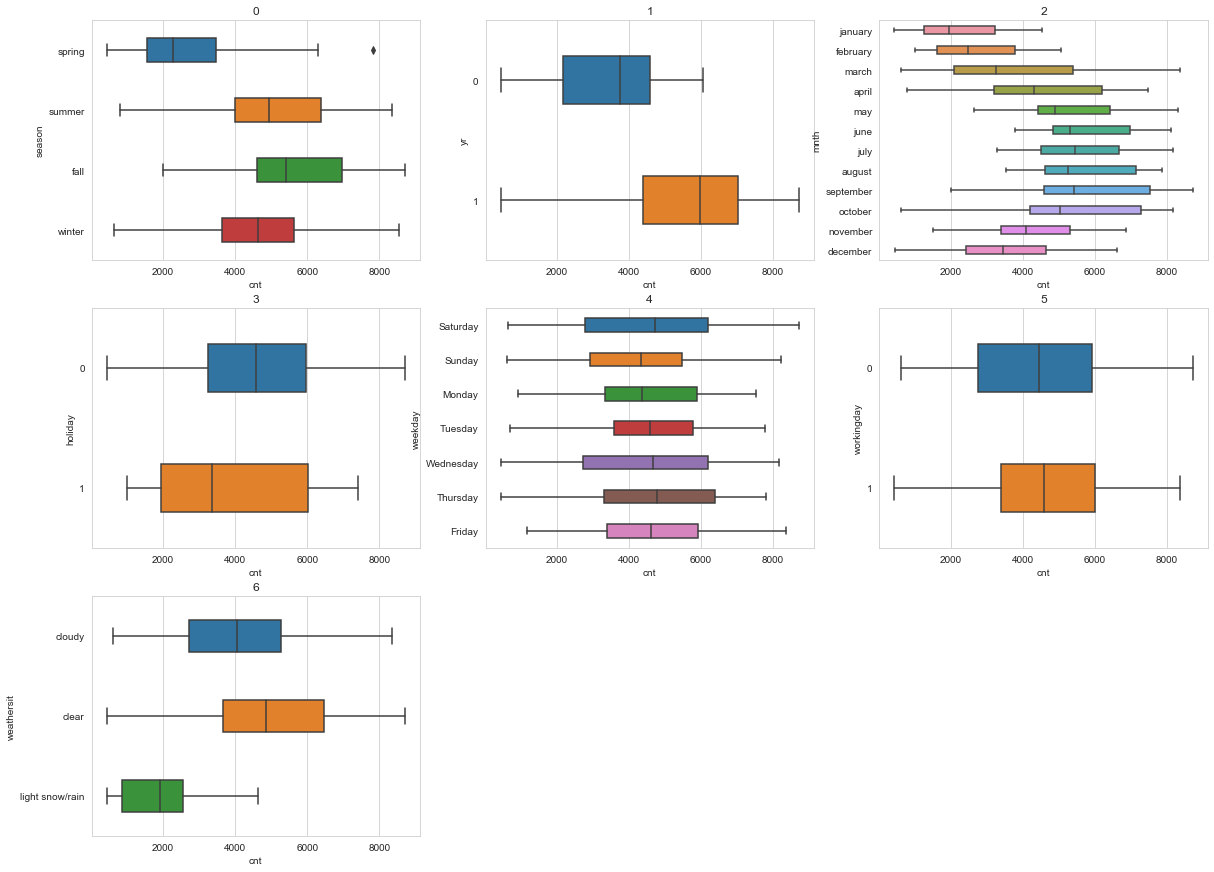
From the season vs rentals per day plot , fall has the highest average rentals followed by summer.
Looking at year by year rentals, 2019 has had a median 2000 increase in rentals compared to 2018.
From the month wise plot, September has the highest rentals, followed by the two months surrounding it. It seems like the trend is explained by seasonal rentals too
Holidays show lower rental count compared to working days, with greater variability in demand on holidays.
There is no significant difference between rentals vs weekdays, except that Thursdays and sundays have a higher variation in rentals than others.

Outliers in Categorical Variables vs cnt

1# Dropping outliers in Categorical Variables
2data = data.drop(index = data[(data['season'] == 'spring') & (data['cnt'] > 7000)].index)

Correlation

1# correlation among variables
2plt.figure(figsize=[10,10])
3sns.heatmap(data.corr(),cmap='GnBu',center=0,annot=True)

1<matplotlib.axes._subplots.AxesSubplot at 0x7fde4bfdd610>

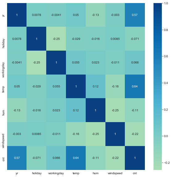
Highest correlation with cnt is seen in temp followed by yr

Data Preparation

Creating Indictor Variables

1# creating indicator variable columns
2season_indicators = pd.get_dummies(data['season'],drop_first=True)
3mnth_indicators = pd.get_dummies(data['mnth'],drop_first=True)
4weekday_indicators = pd.get_dummies(data['weekday'],drop_first=True)
5weathersit_indicators = pd.get_dummies(data['weathersit'],drop_first=True)

1# adding indicator variable columns to the dataset . Dropping original columns
2data = pd.concat([data,season_indicators,mnth_indicators,weekday_indicators,weathersit_indicators],axis=1)
3data = data.drop(columns=['season','mnth','weekday','weathersit'])

1data.head()

1data.columns

1Index(['yr', 'holiday', 'workingday', 'temp', 'hum', 'windspeed', 'cnt',
2       'spring', 'summer', 'winter', 'august', 'december', 'february',
3       'january', 'july', 'june', 'march', 'may', 'november', 'october',
4       'september', 'Monday', 'Saturday', 'Sunday', 'Thursday', 'Tuesday',
5       'Wednesday', 'cloudy', 'light snow/rain'],
6      dtype='object')

Variable	Reference Label
season	fall
mnth	april
weekday	Friday
weathersit	clear

Splitting the data set into Test & Train subsets

1from sklearn.model_selection import train_test_split

1dtrain,dtest = train_test_split(data,train_size=0.7,test_size=0.3,random_state=120)

Scaling Numerical Features

1# normalization of continuous variables
2from sklearn.preprocessing import MinMaxScaler
3numerical_scaler = MinMaxScaler()
4num_vars = ['temp','hum','windspeed']
5
6numerical_scaler.fit(dtrain[num_vars])
7dtrain[num_vars] = numerical_scaler.transform(dtrain[num_vars])

X_train , y_train

1y_train = dtrain.pop('cnt')
2X_train = dtrain

1y_train.head()

1231    5191
2717    5267
3107    3429
4595    4549
5485    5740
6Name: cnt, dtype: int64

1X_train.head()

1X_train.columns

1Index(['yr', 'holiday', 'workingday', 'temp', 'hum', 'windspeed', 'spring',
2       'summer', 'winter', 'august', 'december', 'february', 'january', 'july',
3       'june', 'march', 'may', 'november', 'october', 'september', 'Monday',
4       'Saturday', 'Sunday', 'Thursday', 'Tuesday', 'Wednesday', 'cloudy',
5       'light snow/rain'],
6      dtype='object')

Modelling

Approach

A mixed approach is followed.
15 Best columns are chosen using RFE
And then p-value method is followed for further elimination.

Recursive Feature Elimination

1# Selecting 15 Features using RFE
2
3from sklearn.feature_selection import RFE
4from sklearn.linear_model import LinearRegression
5
6lr_estimator = LinearRegression()
7rfe = RFE(lr_estimator,n_features_to_select=15, step=1)
8selector = rfe.fit(X_train,y_train)

1# RFE Feature Ranking
2rfe_ranking = pd.DataFrame({'rank' : selector.ranking_, 'support': selector.support_, 'features' : X_train.columns}).sort_values(by='rank',ascending=True)
3rfe_ranking

1# Selected Features
2selected_features = rfe_ranking.loc[rfe_ranking['rank'] == 1,'features'].values
3selected_features

1array(['yr', 'Sunday', 'Saturday', 'november', 'january', 'december',
2       'winter', 'july', 'spring', 'holiday', 'workingday', 'hum', 'temp',
3       'windspeed', 'light snow/rain'], dtype=object)

Manual Elimination

1# Following a stepwise elimination
2import statsmodels.api as sm
3def ols_fit(y,X) :
4    X_train_sm = sm.add_constant(X)
5    model = sm.OLS(y,X_train_sm).fit()
6    print(model.summary())
7    return model
8def vif(X) :
9    df = sm.add_constant(X)
10    vif = [variance_inflation_factor(df.values,i) for i in range(df.shape[1])]
11    vif_frame = pd.DataFrame({'vif' : vif[0:]},index = df.columns).reset_index()
12    print(vif_frame.sort_values(by='vif',ascending=False))

Model 1

Using features selected by RFE : ‘yr’, ‘Sunday’, ‘Saturday’, ‘november’, ‘january’, ‘december’, ‘winter’, ‘july’, ‘spring’, ‘holiday’, ‘workingday’, ‘hum’, ‘temp’, ‘windspeed’, ‘light snow/rain’

1features_1 = selected_features
2ols_fit(y_train,X_train[features_1])
3vif(X_train[selected_features])

1OLS Regression Results
2==============================================================================
3Dep. Variable:                    cnt   R-squared:                       0.844
4Model:                            OLS   Adj. R-squared:                  0.840
5Method:                 Least Squares   F-statistic:                     189.8
6Date:                Thu, 30 Jul 2020   Prob (F-statistic):          9.27e-188
7Time:                        20:41:57   Log-Likelihood:                -4072.4
8No. Observations:                 506   AIC:                             8175.
9Df Residuals:                     491   BIC:                             8238.
10Df Model:                          14
11Covariance Type:            nonrobust
12===================================================================================
13                      coef    std err          t      P>|t|      [0.025      0.975]
14-----------------------------------------------------------------------------------
15const            2278.2820    192.838     11.815      0.000    1899.393    2657.171
16yr               1959.7590     69.543     28.180      0.000    1823.120    2096.398
17Sunday            497.0421     97.123      5.118      0.000     306.214     687.871
18Saturday          874.2613     95.093      9.194      0.000     687.422    1061.101
19november         -617.4927    158.994     -3.884      0.000    -929.885    -305.100
20january          -391.9320    149.160     -2.628      0.009    -685.002     -98.862
21december         -475.8630    142.634     -3.336      0.001    -756.112    -195.614
22winter            687.2832    121.588      5.653      0.000     448.387     926.180
23july             -804.3128    141.415     -5.688      0.000   -1082.166    -526.459
24spring          -1010.6061    134.437     -7.517      0.000   -1274.749    -746.464
25holiday           165.4153    160.101      1.033      0.302    -149.152     479.982
26workingday        741.5633     73.655     10.068      0.000     596.846     886.280
27hum             -1782.6033    198.667     -8.973      0.000   -2172.947   -1392.260
28temp             4036.2727    275.497     14.651      0.000    3494.974    4577.571
29windspeed       -1167.6983    188.628     -6.190      0.000   -1538.315    -797.081
30light snow/rain -1276.7947    234.425     -5.446      0.000   -1737.395    -816.194
31==============================================================================
32Omnibus:                       74.940   Durbin-Watson:                   1.920
33Prob(Omnibus):                  0.000   Jarque-Bera (JB):              164.191
34Skew:                          -0.800   Prob(JB):                     2.22e-36
35Kurtosis:                       5.286   Cond. No.                     6.67e+15
36==============================================================================
37
38Warnings:
39[1] Standard Errors assume that the covariance matrix of the errors is correctly specified.
40[2] The smallest eigenvalue is 3.03e-29. This might indicate that there are
41strong multicollinearity problems or that the design matrix is singular.
42              index       vif
432            Sunday       inf
443          Saturday       inf
4510          holiday       inf
4611       workingday       inf
4713             temp  3.530342
489            spring  2.972066
497            winter  2.265754
505           january  1.667765
514          november  1.649107
526          december  1.384399
538              july  1.332786
5412              hum  1.302061
5515  light snow/rain  1.179013
5614        windspeed  1.161178
571                yr  1.035227
580             const  0.000000

Model 2 :

Dropping holiday because of high p-value

1del_feature = 'holiday'
2selected_features = selected_features[selected_features!=del_feature]
3ols_fit(y_train,X_train[selected_features])
4vif(X_train[selected_features])

1OLS Regression Results
2==============================================================================
3Dep. Variable:                    cnt   R-squared:                       0.844
4Model:                            OLS   Adj. R-squared:                  0.840
5Method:                 Least Squares   F-statistic:                     189.8
6Date:                Thu, 30 Jul 2020   Prob (F-statistic):          9.27e-188
7Time:                        20:41:57   Log-Likelihood:                -4072.4
8No. Observations:                 506   AIC:                             8175.
9Df Residuals:                     491   BIC:                             8238.
10Df Model:                          14
11Covariance Type:            nonrobust
12===================================================================================
13                      coef    std err          t      P>|t|      [0.025      0.975]
14-----------------------------------------------------------------------------------
15const            2443.6973    302.113      8.089      0.000    1850.103    3037.291
16yr               1959.7590     69.543     28.180      0.000    1823.120    2096.398
17Sunday            331.6268    208.945      1.587      0.113     -78.910     742.164
18Saturday          708.8460    208.062      3.407      0.001     300.043    1117.649
19november         -617.4927    158.994     -3.884      0.000    -929.885    -305.100
20january          -391.9320    149.160     -2.628      0.009    -685.002     -98.862
21december         -475.8630    142.634     -3.336      0.001    -756.112    -195.614
22winter            687.2832    121.588      5.653      0.000     448.387     926.180
23july             -804.3128    141.415     -5.688      0.000   -1082.166    -526.459
24spring          -1010.6061    134.437     -7.517      0.000   -1274.749    -746.464
25workingday        576.1480    191.468      3.009      0.003     199.950     952.346
26hum             -1782.6033    198.667     -8.973      0.000   -2172.947   -1392.260
27temp             4036.2727    275.497     14.651      0.000    3494.974    4577.571
28windspeed       -1167.6983    188.628     -6.190      0.000   -1538.315    -797.081
29light snow/rain -1276.7947    234.425     -5.446      0.000   -1737.395    -816.194
30==============================================================================
31Omnibus:                       74.940   Durbin-Watson:                   1.920
32Prob(Omnibus):                  0.000   Jarque-Bera (JB):              164.191
33Skew:                          -0.800   Prob(JB):                     2.22e-36
34Kurtosis:                       5.286   Cond. No.                         20.6
35==============================================================================
36
37Warnings:
38[1] Standard Errors assume that the covariance matrix of the errors is correctly specified.
39              index        vif
400             const  78.227579
4110       workingday   6.747604
423          Saturday   4.580552
432            Sunday   4.352788
4412             temp   3.530342
459            spring   2.972066
467            winter   2.265754
475           january   1.667765
484          november   1.649107
496          december   1.384399
508              july   1.332786
5111              hum   1.302061
5214  light snow/rain   1.179013
5313        windspeed   1.161178
541                yr   1.035227

Model 3 :

Dropping Sunday because of high p-value

1del_feature = 'Sunday'
2selected_features = selected_features[selected_features!=del_feature]
3ols_fit(y_train,X_train[selected_features])
4vif(X_train[selected_features])

1OLS Regression Results
2==============================================================================
3Dep. Variable:                    cnt   R-squared:                       0.843
4Model:                            OLS   Adj. R-squared:                  0.839
5Method:                 Least Squares   F-statistic:                     203.6
6Date:                Thu, 30 Jul 2020   Prob (F-statistic):          2.22e-188
7Time:                        20:41:57   Log-Likelihood:                -4073.7
8No. Observations:                 506   AIC:                             8175.
9Df Residuals:                     492   BIC:                             8234.
10Df Model:                          13
11Covariance Type:            nonrobust
12===================================================================================
13                      coef    std err          t      P>|t|      [0.025      0.975]
14-----------------------------------------------------------------------------------
15const            2717.6842    248.317     10.944      0.000    2229.791    3205.578
16yr               1958.8083     69.648     28.124      0.000    1821.964    2095.652
17Saturday          442.9774    123.597      3.584      0.000     200.134     685.820
18november         -627.3327    159.118     -3.943      0.000    -939.968    -314.698
19january          -391.6152    149.390     -2.621      0.009    -685.136     -98.095
20december         -485.7607    142.718     -3.404      0.001    -766.172    -205.350
21winter            687.9955    121.774      5.650      0.000     448.733     927.258
22july             -808.0743    141.613     -5.706      0.000   -1086.316    -529.833
23spring          -1018.8530    134.544     -7.573      0.000   -1283.204    -754.502
24workingday        310.9383     93.623      3.321      0.001     126.989     494.888
25hum             -1777.8858    198.952     -8.936      0.000   -2168.785   -1386.986
26temp             4023.0506    275.796     14.587      0.000    3481.168    4564.933
27windspeed       -1166.7398    188.918     -6.176      0.000   -1537.925    -795.555
28light snow/rain -1274.2371    234.781     -5.427      0.000   -1735.535    -812.939
29==============================================================================
30Omnibus:                       76.586   Durbin-Watson:                   1.907
31Prob(Omnibus):                  0.000   Jarque-Bera (JB):              168.964
32Skew:                          -0.814   Prob(JB):                     2.04e-37
33Kurtosis:                       5.316   Cond. No.                         17.6
34==============================================================================
35
36Warnings:
37[1] Standard Errors assume that the covariance matrix of the errors is correctly specified.
38              index        vif
390             const  52.686107
4011             temp   3.527114
418            spring   2.967626
426            winter   2.265723
434           january   1.667762
443          november   1.646599
452          Saturday   1.611416
469        workingday   1.608346
475          december   1.381753
487              july   1.332412
4910              hum   1.301769
5013  light snow/rain   1.178957
5112        windspeed   1.161167
521                yr   1.035151

Model 4

Dropping january because this information might also be contained in winter.

1del_feature = 'january'
2selected_features = selected_features[selected_features!=del_feature]
3ols_fit(y_train,X_train[selected_features])
4vif(X_train[selected_features])

1OLS Regression Results
2==============================================================================
3Dep. Variable:                    cnt   R-squared:                       0.841
4Model:                            OLS   Adj. R-squared:                  0.837
5Method:                 Least Squares   F-statistic:                     217.4
6Date:                Thu, 30 Jul 2020   Prob (F-statistic):          4.41e-188
7Time:                        20:41:58   Log-Likelihood:                -4077.2
8No. Observations:                 506   AIC:                             8180.
9Df Residuals:                     493   BIC:                             8235.
10Df Model:                          12
11Covariance Type:            nonrobust
12===================================================================================
13                      coef    std err          t      P>|t|      [0.025      0.975]
14-----------------------------------------------------------------------------------
15const            2563.5282    242.686     10.563      0.000    2086.701    3040.355
16yr               1951.9279     70.012     27.880      0.000    1814.370    2089.486
17Saturday          437.2585    124.312      3.517      0.000     193.013     681.504
18november         -576.6481    158.877     -3.630      0.000    -888.808    -264.489
19december         -380.3554    137.749     -2.761      0.006    -651.004    -109.707
20winter            696.8818    122.450      5.691      0.000     456.294     937.470
21july             -846.1814    141.702     -5.972      0.000   -1124.595    -567.768
22spring          -1101.5863    131.566     -8.373      0.000   -1360.086    -843.087
23workingday        310.1011     94.178      3.293      0.001     125.061     495.141
24hum             -1775.7238    200.131     -8.873      0.000   -2168.939   -1382.508
25temp             4232.4252    265.545     15.939      0.000    3710.686    4754.164
26windspeed       -1126.2015    189.402     -5.946      0.000   -1498.335    -754.068
27light snow/rain -1259.9614    236.112     -5.336      0.000   -1723.871    -796.052
28==============================================================================
29Omnibus:                       70.215   Durbin-Watson:                   1.923
30Prob(Omnibus):                  0.000   Jarque-Bera (JB):              144.730
31Skew:                          -0.775   Prob(JB):                     3.74e-32
32Kurtosis:                       5.112   Cond. No.                         16.9
33==============================================================================
34
35Warnings:
36[1] Standard Errors assume that the covariance matrix of the errors is correctly specified.
37              index        vif
380             const  49.731331
3910             temp   3.231303
407            spring   2.804334
415            winter   2.263968
423          november   1.622287
432          Saturday   1.610914
448        workingday   1.608327
456              july   1.318372
469               hum   1.301747
474          december   1.272074
4812  light snow/rain   1.178323
4911        windspeed   1.153386
501                yr   1.033680

Model 5

Dropping december because this information might also be contained in winter.

1del_feature = 'december'
2selected_features = selected_features[selected_features!=del_feature]
3ols_fit(y_train,X_train[selected_features])
4vif(X_train[selected_features])

1OLS Regression Results
2==============================================================================
3Dep. Variable:                    cnt   R-squared:                       0.839
4Model:                            OLS   Adj. R-squared:                  0.835
5Method:                 Least Squares   F-statistic:                     233.3
6Date:                Thu, 30 Jul 2020   Prob (F-statistic):          1.22e-187
7Time:                        20:41:58   Log-Likelihood:                -4081.1
8No. Observations:                 506   AIC:                             8186.
9Df Residuals:                     494   BIC:                             8237.
10Df Model:                          11
11Covariance Type:            nonrobust
12===================================================================================
13                      coef    std err          t      P>|t|      [0.025      0.975]
14-----------------------------------------------------------------------------------
15const            2484.0272    242.583     10.240      0.000    2007.406    2960.648
16yr               1945.4495     70.440     27.619      0.000    1807.051    2083.848
17Saturday          435.8371    125.141      3.483      0.001     189.962     681.712
18november         -443.0313    152.340     -2.908      0.004    -742.345    -143.718
19winter            603.4461    118.468      5.094      0.000     370.683     836.209
20july             -874.0132    142.287     -6.143      0.000   -1153.576    -594.450
21spring          -1106.1972    132.435     -8.353      0.000   -1366.402    -845.992
22workingday        296.4789     94.677      3.131      0.002     110.459     482.499
23hum             -1801.9289    201.242     -8.954      0.000   -2197.325   -1406.533
24temp             4372.9630    262.363     16.668      0.000    3857.478    4888.448
25windspeed       -1096.9814    190.369     -5.762      0.000   -1471.015    -722.948
26light snow/rain -1259.4132    237.690     -5.299      0.000   -1726.420    -792.406
27==============================================================================
28Omnibus:                       67.769   Durbin-Watson:                   1.914
29Prob(Omnibus):                  0.000   Jarque-Bera (JB):              129.549
30Skew:                          -0.778   Prob(JB):                     7.39e-29
31Kurtosis:                       4.929   Cond. No.                         16.7
32==============================================================================
33
34Warnings:
35[1] Standard Errors assume that the covariance matrix of the errors is correctly specified.
36              index        vif
370             const  49.031354
389              temp   3.112593
396            spring   2.803882
404            winter   2.091074
412          Saturday   1.610886
427        workingday   1.603914
433          november   1.471790
445              july   1.311701
458               hum   1.298820
4611  light snow/rain   1.178322
4710        windspeed   1.149786
481                yr   1.032520

Model 6

Dropping november because this information might also be contained in winter.

1del_feature = 'november'
2selected_features = selected_features[selected_features!=del_feature]
3final_model = ols_fit(y_train,X_train[selected_features])
4vif(X_train[selected_features])

1OLS Regression Results
2==============================================================================
3Dep. Variable:                    cnt   R-squared:                       0.836
4Model:                            OLS   Adj. R-squared:                  0.833
5Method:                 Least Squares   F-statistic:                     252.0
6Date:                Thu, 30 Jul 2020   Prob (F-statistic):          4.89e-187
7Time:                        20:41:58   Log-Likelihood:                -4085.3
8No. Observations:                 506   AIC:                             8193.
9Df Residuals:                     495   BIC:                             8239.
10Df Model:                          10
11Covariance Type:            nonrobust
12===================================================================================
13                      coef    std err          t      P>|t|      [0.025      0.975]
14-----------------------------------------------------------------------------------
15const            2392.0791    242.318      9.872      0.000    1915.980    2868.178
16yr               1946.7864     70.967     27.432      0.000    1807.353    2086.220
17Saturday          444.4907    126.045      3.526      0.000     196.842     692.139
18winter            466.0136    109.450      4.258      0.000     250.970     681.057
19july             -890.3115    143.244     -6.215      0.000   -1171.752    -608.871
20spring          -1063.6669    132.613     -8.021      0.000   -1324.220    -803.114
21workingday        296.8008     95.388      3.112      0.002     109.386     484.216
22hum             -1749.8275    201.947     -8.665      0.000   -2146.607   -1353.048
23temp             4471.6602    262.111     17.060      0.000    3956.673    4986.648
24windspeed       -1110.3191    191.742     -5.791      0.000   -1487.049    -733.590
25light snow/rain -1273.7519    239.422     -5.320      0.000   -1744.160    -803.344
26==============================================================================
27Omnibus:                       69.587   Durbin-Watson:                   1.898
28Prob(Omnibus):                  0.000   Jarque-Bera (JB):              136.276
29Skew:                          -0.788   Prob(JB):                     2.56e-30
30Kurtosis:                       4.995   Cond. No.                         16.5
31==============================================================================
32
33Warnings:
34[1] Standard Errors assume that the covariance matrix of the errors is correctly specified.
35              index        vif
360             const  48.198446
378              temp   3.060511
385            spring   2.769692
393            winter   1.758336
402          Saturday   1.609975
416        workingday   1.603912
424              july   1.309666
437               hum   1.288526
4410  light snow/rain   1.177815
459         windspeed   1.149118
461                yr   1.032476

Verifying MultiCollinearity

1vif(X_train[selected_features])

1index        vif
20             const  48.198446
38              temp   3.060511
45            spring   2.769692
53            winter   1.758336
62          Saturday   1.609975
76        workingday   1.603912
84              july   1.309666
97               hum   1.288526
1010  light snow/rain   1.177815
119         windspeed   1.149118
121                yr   1.032476

VIF < 5 for selected features. No significant multicollinearity observed. Similar indicating comparison of R-squared and adjusted R-squared.

Final Model

1final_model = ols_fit(y_train,X_train[selected_features])

1OLS Regression Results
2==============================================================================
3Dep. Variable:                    cnt   R-squared:                       0.836
4Model:                            OLS   Adj. R-squared:                  0.833
5Method:                 Least Squares   F-statistic:                     252.0
6Date:                Thu, 30 Jul 2020   Prob (F-statistic):          4.89e-187
7Time:                        20:41:58   Log-Likelihood:                -4085.3
8No. Observations:                 506   AIC:                             8193.
9Df Residuals:                     495   BIC:                             8239.
10Df Model:                          10
11Covariance Type:            nonrobust
12===================================================================================
13                      coef    std err          t      P>|t|      [0.025      0.975]
14-----------------------------------------------------------------------------------
15const            2392.0791    242.318      9.872      0.000    1915.980    2868.178
16yr               1946.7864     70.967     27.432      0.000    1807.353    2086.220
17Saturday          444.4907    126.045      3.526      0.000     196.842     692.139
18winter            466.0136    109.450      4.258      0.000     250.970     681.057
19july             -890.3115    143.244     -6.215      0.000   -1171.752    -608.871
20spring          -1063.6669    132.613     -8.021      0.000   -1324.220    -803.114
21workingday        296.8008     95.388      3.112      0.002     109.386     484.216
22hum             -1749.8275    201.947     -8.665      0.000   -2146.607   -1353.048
23temp             4471.6602    262.111     17.060      0.000    3956.673    4986.648
24windspeed       -1110.3191    191.742     -5.791      0.000   -1487.049    -733.590
25light snow/rain -1273.7519    239.422     -5.320      0.000   -1744.160    -803.344
26==============================================================================
27Omnibus:                       69.587   Durbin-Watson:                   1.898
28Prob(Omnibus):                  0.000   Jarque-Bera (JB):              136.276
29Skew:                          -0.788   Prob(JB):                     2.56e-30
30Kurtosis:                       4.995   Cond. No.                         16.5
31==============================================================================
32
33Warnings:
34[1] Standard Errors assume that the covariance matrix of the errors is correctly specified.

10 features have been selected.
All the features are statistically significant [low p-value]
The model over is a good fit with Prob (F-statistic): 4.89e-187
The model explains 83.6% variability in the training data. Adjusted R-square being 83.3%

Residual Analysis

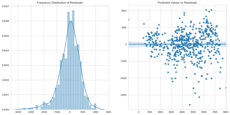
1# Residual Analysis of Trained Data
2X_train_sm = sm.add_constant(X_train[selected_features])
3
4y_train_pred = final_model.predict(X_train_sm)
5fig,ax = plt.subplots(1,2)
6fig.set_figheight(8)
7fig.set_figwidth(16)
8
9ax[0].set(title='Frequency Distribution of Residuals')
10sns.distplot(y_train-y_train_pred, bins=30, ax=ax[0])
11
12ax[1].set(title='Predicted Values vs Residuals')
13\
14sns.regplot(y_train_pred,y_train-y_train_pred,ax=ax[1])
15plt.show()

1# Mean of Residuals
2(y_train-y_train_pred).mean()

14.763163951972846e-12

Residual errors follow a normal distribution with mean=0
Variance of Errors doesnt follow any trends
Residual errors are independent of each other since the Predicted values vs Residuals plot doesn’t show any trend.

1# Verifying the normality of distribution of residuals
2mean = (y_train-y_train_pred).mean()
3std = (y_train-y_train_pred).std()
4
5ref_normal = np.random.normal(mean,std,(y_train-y_train_pred).shape[0])
6
7
8percs = np.linspace(0,100,21)
9qn_ref_normal = np.percentile(ref_normal, percs)
10qn_residual = np.percentile(y_train - y_train_pred , percs)
11
12plt.plot(qn_ref_normal,qn_residual, ls="", marker="o")
13
14x = np.linspace(np.min((qn_ref_normal.min(),qn_residual.min())), np.max((qn_ref_normal.max(),qn_residual.max())))
15m = plt.plot(x,x, color="k", ls="--")
16plt.title('Q-Q Plot : Reference Normal vs Distribution of Residuals ')
17plt.savefig('q-q-plot.png')
18plt.show()

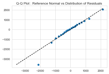
This plot further shows that the residual distribution is approximately normal for all test data with values within range of training data.

1# lag plot to assess independence of data points
2from pandas.plotting import lag_plot
3lag_plot(y_train-y_train_pred)

1<matplotlib.axes._subplots.AxesSubplot at 0x7fde4fb985d0>

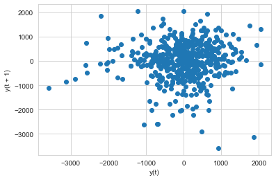
Lagplot of residuals shows no trend. Hence the error terms have constant variance

Hence, assumptions of Linear Regression are satisfied by this model

Prediction

1y_test = dtest.pop('cnt')
2X_test = dtest
3X_test[num_vars] = numerical_scaler.transform(X_test[num_vars])
4X_test = X_test[selected_features]

1X_test = sm.add_constant(X_test)
2y_test_pred = final_model.predict(X_test)

Model Evaluation

1# Plotting Actual vs Predicted No of rentals
2fig,ax = plt.subplots()
3fig.set_figheight(8)
4fig.set_figwidth(20)
5l1,=ax.plot(range(len(y_test)),y_test)
6l2, = ax.plot(range(len(y_test_pred)),y_test_pred)
7plt.legend([l1,l2],['Actual','Predicted'])
8plt.title('Predicted vs Actual No of Rentals');
9plt.ylabel('No of Bike Rentals')
10plt.xticks([])
11plt.show()
12
13plt.figure(figsize=[8,8])
14plt.scatter(y_test,y_test_pred);
15plt.title('Predicted vs Actual No of Rentals');

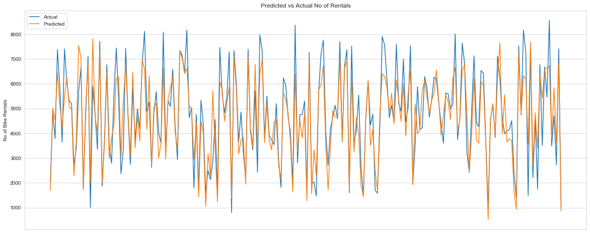
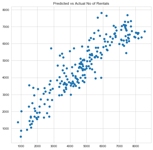
Predicted vs observed value plots shows that the model is reasonably accurate.

1from sklearn.metrics import mean_squared_error,r2_score
2mse = mean_squared_error(y_test, y_test_pred)
3rsquared_test = r2_score(y_test, y_test_pred)
4rsquared_train = r2_score(y_train, y_train_pred)
5print('R-squared for train data:',round(rsquared_train,2))
6print('R-squared for test data:',round(rsquared_test,2))
7print('Mean Squared Error',round(mse,3))

1R-squared for train data: 0.84
2R-squared for test data: 0.81
3Mean Squared Error 666097.695

Model Stability

1# R-square using cross validation
2
3from sklearn.model_selection import cross_val_score
4from sklearn.linear_model import LinearRegression
5lr = LinearRegression()
6clr = cross_val_score(lr,X_train[selected_features],y_train,cv=10, scoring='r2')
7clr

1array([0.76577509, 0.89378885, 0.73439962, 0.87831664, 0.84127272,
2       0.85375903, 0.87521829, 0.68697543, 0.73861901, 0.87571386])

1print("R-square at 0.95 confidence level : %0.2f (+/- %0.2f)" % (clr.mean(), clr.std() * 2))

1R-square at 0.95 confidence level : 0.81 (+/- 0.14)

1selected_features

1array(['yr', 'Saturday', 'winter', 'july', 'spring', 'workingday', 'hum',
2       'temp', 'windspeed', 'light snow/rain'], dtype=object)

Top Features

1# standardizing numerical variables
2
3from sklearn.preprocessing import StandardScaler
4reg_features = selected_features
5scaler = StandardScaler()
6data = X_train[selected_features]
7std_num = scaler.fit(data[['temp','windspeed','hum']])
8
9
10std_X_train = pd.DataFrame(data = scaler.transform(data[['temp','windspeed','hum']]), columns=['temp','windspeed','hum'])
11for i in reg_features :
12    std_X_train[i] = data[i].values
13
14
15reshaped_y_train = y_train.values.reshape(-1,1)
16
17# Fitting linear regression model
18std_model = lr.fit(std_X_train, reshaped_y_train)
19
20# Coefficients and intercept
21result = pd.DataFrame(data = std_model.coef_, columns = std_X_train.columns, index=['MLR Coefficients']).T
22result = result.sort_values(by='MLR Coefficients',ascending=False)
23print('\nIntercept :',std_model.intercept_)
24result

1Intercept : [2392.07911232]

Upon standardized the values of predictor variables, the above shows that the top features influencing demand are temp, followed by yr and hum
In case of continuous variables, the above data could be interpreted as - With every standard deviation increase in continuous variables, demand increases by xxx, when all other modelled paramters are held unchanged.
In case of categorical variables, the above data could be interpreted as - Compared to the reference level, the change in demand is xxx,, when all other modelled paramters are held unchanged.

Conclusion

cnt = 2392.0791 + 1946.7864 yr + 444.4907 Saturday + 466.0136 winter - 890.3115 july -1063.6669 spring + 296.8008 workingday - 1749.8275 hum + 4471.6602 temp - 1110.3191 windspeed - 1273.7519 light snow/rain